R programming for beginners (GV900)

Lesson 9: Normal distribution ~ Part 2

Friday, January 12, 2024

Video of Lesson 9

1 Setup

In last lesson, we learned the basic concept of normal distribution, which is about what is normal distribution. In this lesson, we will learn how to use normal distribution to solve problems.

First, load the packages we will use in this lesson.

Code

library(tidyverse)
library(openintro)
library(gapminder)

2 Find out the probability of the data

Unlike discrete data, the y axis in continuous data does not represent the probability of the data.
We can only use the area under the curve to describe the probability of the continuous data.
We can use CDF (Cumulative Distribution Function) to calculate the probability of the data.
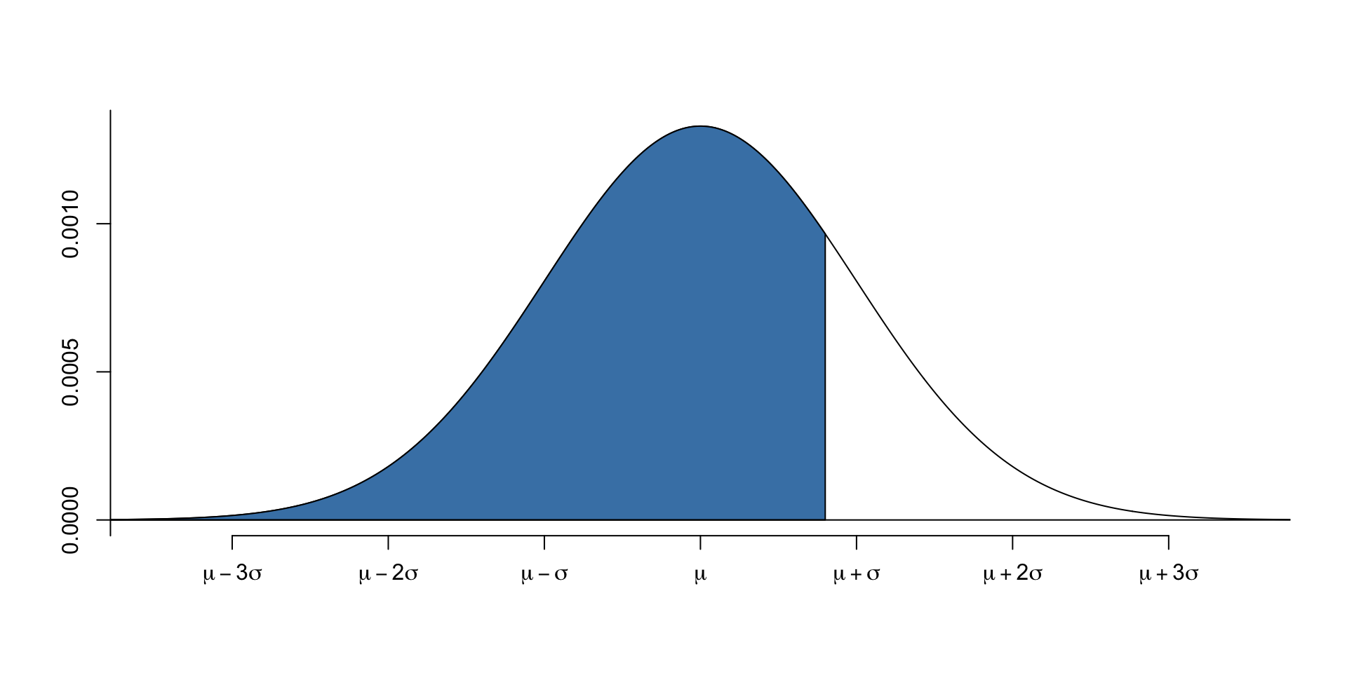
\(F(x)\) represent the probability of the data less than x, i.e., the area under the curve to the left of x.
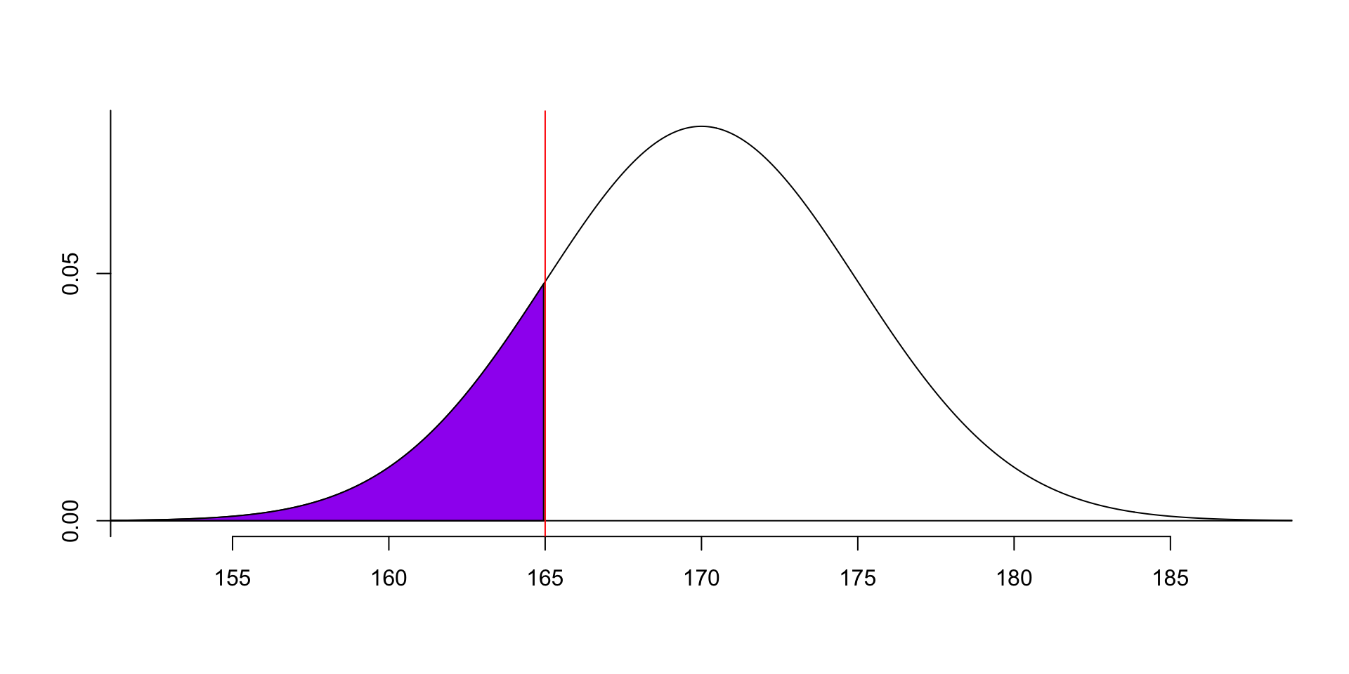
For example, we can calculate the probability of the data is less than 165: \(F(165) = P(x<165) = ?\).

Code

normTail(m = 170, # mean
         s = 5, # standard deviation
         L = 165, # lower range
         col = "purple",
         axes = 3)
# add a vertical line to show the mean
abline(v = 165, col = "red")

We can use R function to find out the probability easily.

Code

pnorm(q = 165, mean = 170, sd = 5)

[1] 0.1586553

- The first argument is the value of the data.
- The second argument is the mean of the data.
- The third argument is the standard deviation of the data.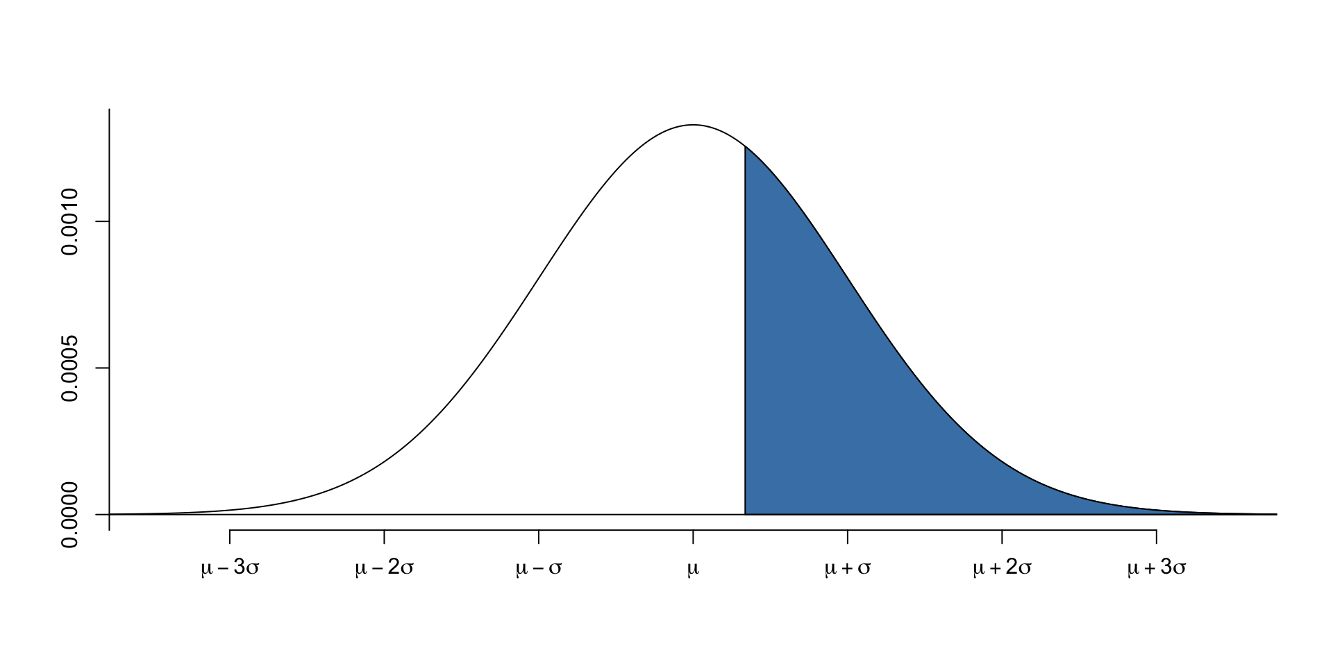
- This example shows that the probability of the data is less than 165 is 0.1587, i.e. 15.87%.

We can also calculate the probability of the data is greater than 165: \(P(x>165) =?\).

Code

normTail(m = 170, # mean
         s = 5, # standard deviation
         U = 165, # lower range
         col = "purple",
         axes = 3)
# add a vertical line to show the mean
abline(v = 165, col = "red")

Code

pnorm(q = 165, mean = 170, sd = 5, lower.tail = FALSE)

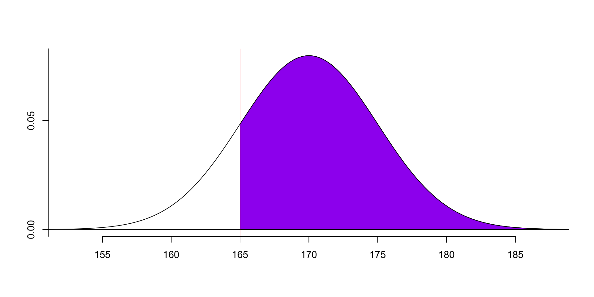
[1] 0.8413447

\(lower.tail = FALSE\) means that we want to calculate the probability of the data greater than 165.
This example shows that the probability of the data is greater than 165 is 0.8413, i.e. 84.13%.
Actually, since the total area under the curve is 1, we can calculate the probability of the data greater than 165 by subtracting the probability of the data is less than 165 from 1: \(P(x>165) = 1 - P(x<165) = 1 - F(165)\).

Code

1 - pnorm(q = 165, mean = 170, sd = 5)

[1] 0.8413447

No surprise, the result is the same as the above.
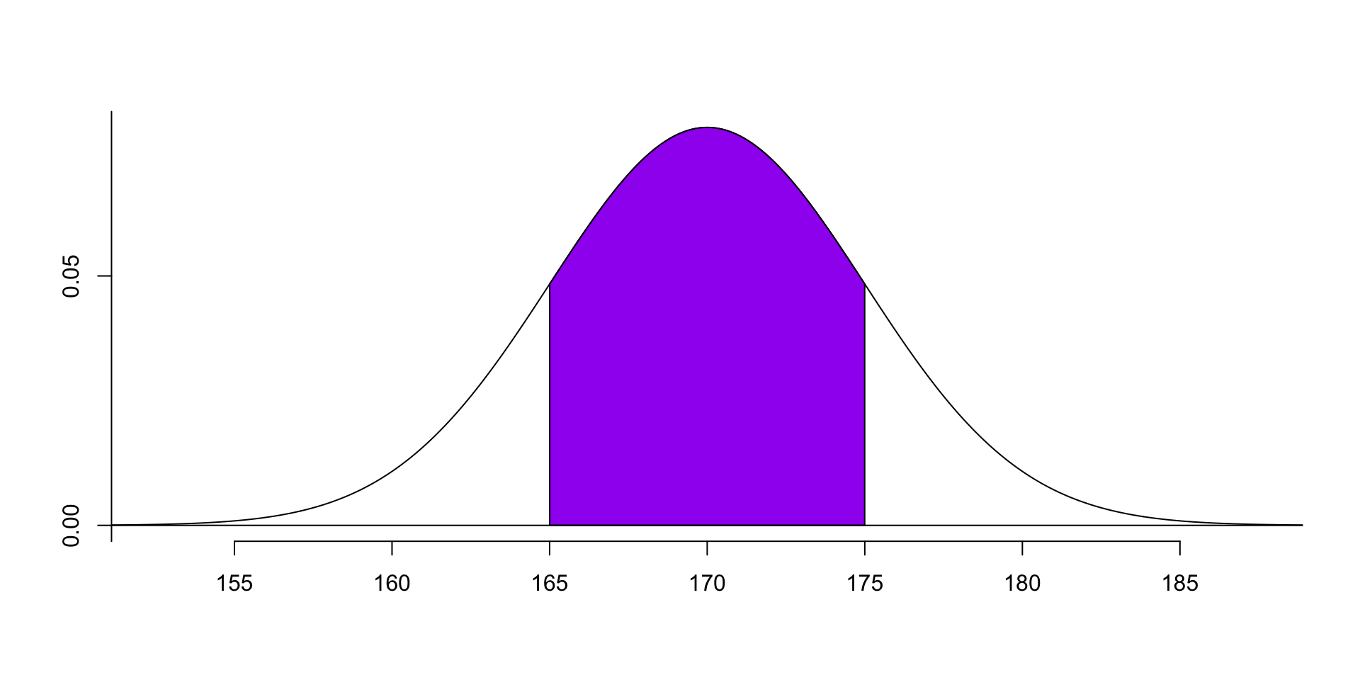
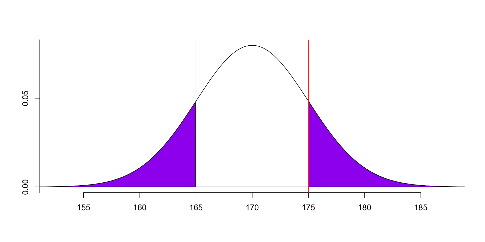
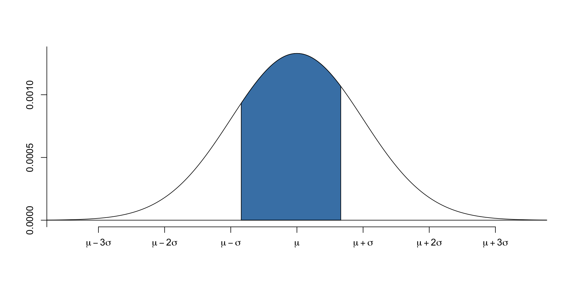
We can also calculate the probability of the data is between 165 and 175: \(P(165<x<175) = ?\).

Code

normTail(m = 170, # mean
         s = 5, # standard deviation
         M = c(165, 175), # middle range
         col = "purple",
         axes = 3)

We have plenty of ways to calculate it.
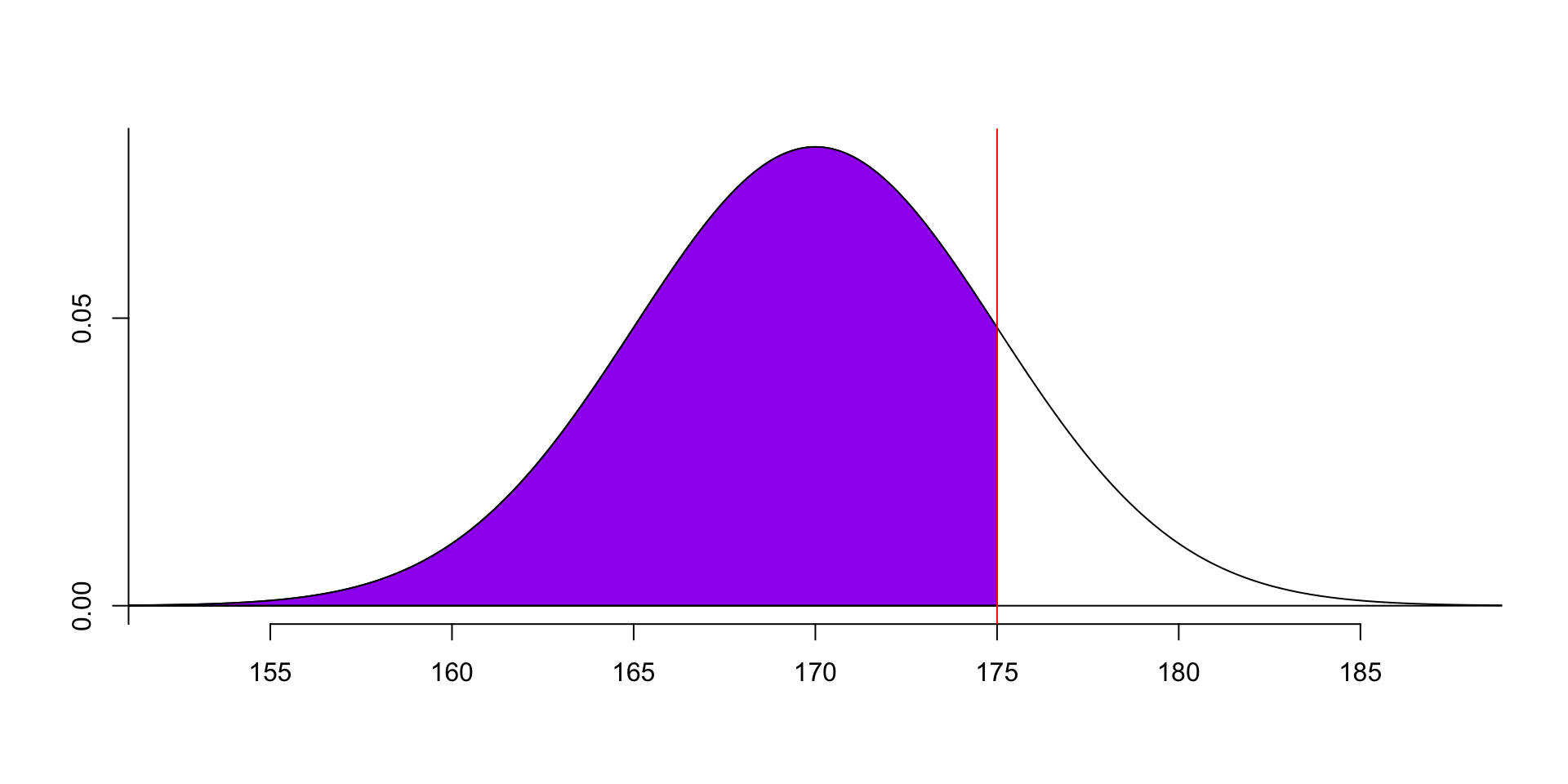
We can calculate the probability of the data less than 175 first, then subtract the probability of the data less than 165 from it: \(P(165<x<175) = P(x<175) - P(x<165) = F(175) - F(165)\).
i.e., we use the area of the following purple part:

Code

normTail(m = 170, # mean
         s = 5, # standard deviation
         L = 175, 
         col = "purple",
         axes = 3)
abline(v = 175, col = "red")

minus the area of this part:

Code

normTail(m = 170, # mean
         s = 5, # standard deviation
         L = 165, # lower range
         col = "purple",
         axes = 3)
abline(v = 165, col = "red")

In R, we can use the following formula to calculate it.

Code

pnorm(q = 175, mean = 170, sd = 5) - pnorm(q = 165, mean = 170, sd = 5)

[1] 0.6826895

This example shows that the probability of the data between 165 and 175 is 0.6827, i.e. 68.27%.
Remember that the total area under the curve is 1, so the probability of the data between 165 and 175 is 1 minus the probability of the data less than 165 and greater than 175: \(P(165<x<175) = 1 - P(x<165) - P(x>175) = 1 - F(165) - (1 - F(175))\).
So we can use 1 minus the following two parts to calculate it.

Code

normTail(m = 170, # mean
         s = 5, # standard deviation
         L = 165, # lower range
         U = 175, # upper range
         col = "purple",
         axes = 3)
abline(v = 165, col = "red")
abline(v = 175, col = "red")

In r, it would be like this:

Code

1 - pnorm(q = 165, mean = 170, sd = 5) - pnorm(q = 175, mean = 170, sd = 5, lower.tail = FALSE)

[1] 0.6826895

No surprise, the result is the same as the above.
Remember that the normal distribution is symmetrically distributed around the mean, so the probability of the data less than 165 is the same as the probability of the data greater than 175, because the distances from 165 and 175 to 170 is the same: \(P(x<165<175) = 1 - 2 \times P(x<165)\).

Code

normTail(m = 170, # mean
         s = 5, # standard deviation
         L = 165, # lower range
         U = 175, # upper range
         col = "purple",
         axes = 3)
abline(v = 170, col = "red")

So, we can use the following formula to calculate the probability even simpler.

Code

1 - 2 * pnorm(q = 165, mean = 170, sd = 5)

[1] 0.6826895

Again, the result is the same as the above two.

3 Find out the critical value if we know the probability

We can also use CDF to find out the critical value if we know the probability.

First, understand the 68-95-99.7 rule.

- 68% of the data is within 1 standard deviation of the mean.

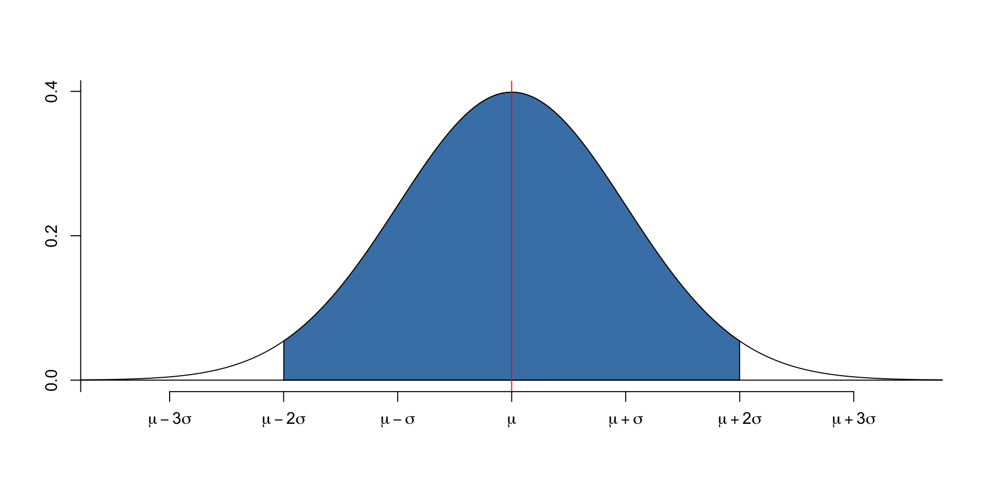
- 95% of the data is within 2 standard deviations of the mean.

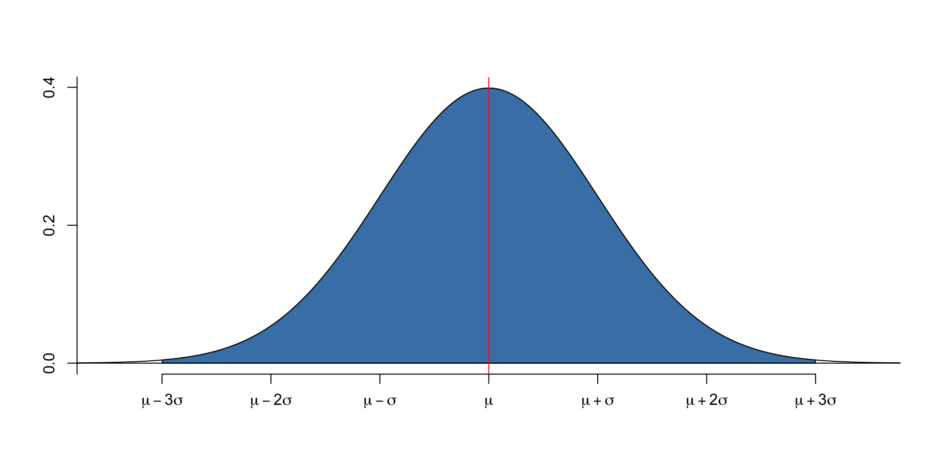
- 99.7% of the data is within 3 standard deviations of the mean.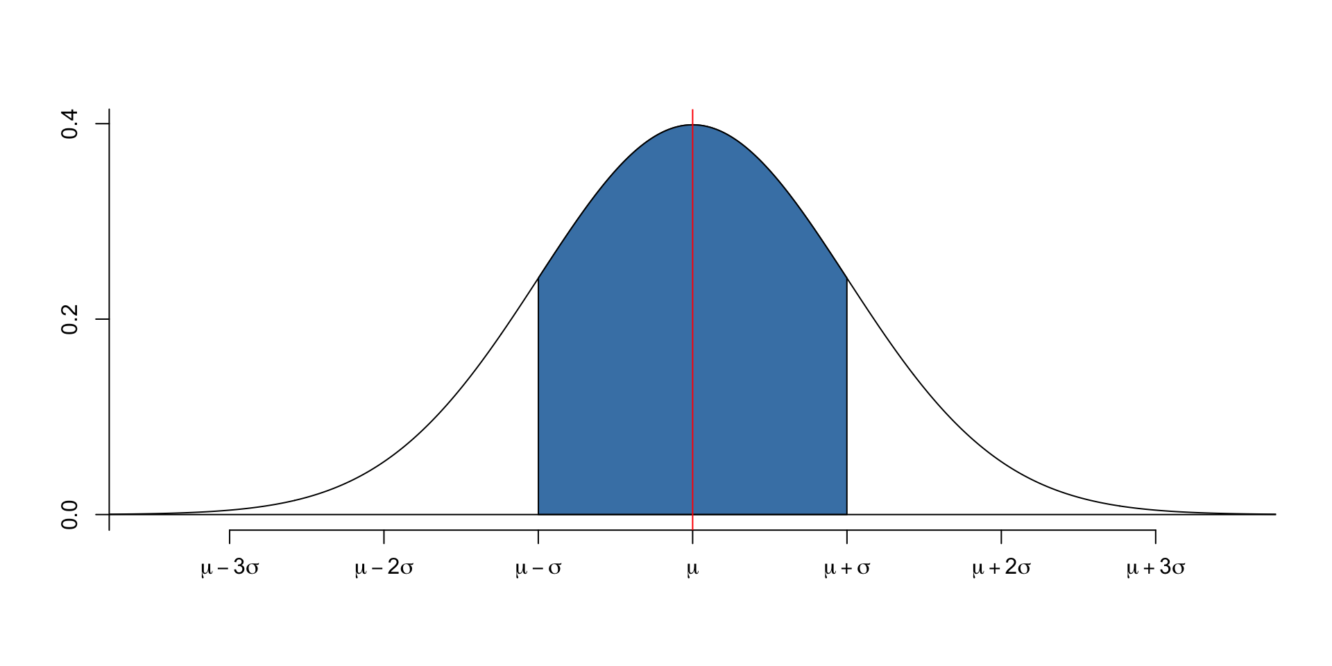

68% rule
95% rule
99.7% rule

Code

normTail(m = 0, # mean
         s = 1, # standard deviation
         M = c(-1, 1), # range
         col = "steelblue",
         axes = 3,
         xLab = "symbol")
abline(v = 0, col = "red")

Code

# standard normal distribution: 95% of the data is within 2 standard deviations of the mean
normTail(m = 0, # mean
         s = 1, # standard deviation
         M = c(-2, 2), # range
         col = "steelblue",
         axes = 3,
         xLab = "symbol")
abline(v = 0, col = "red")

Code

# standard normal distribution: 99.7% of the data is within 3 standard deviations of the mean
normTail(m = 0, # mean
         s = 1, # standard deviation
         M = c(-3, 3), # range
         col = "steelblue",
         axes = 3,
         xLab = "symbol")
abline(v = 0, col = "red")

qnorm() function

If it is not exactly the above probability, we can easily use R function qnorm() to find out the critical value.

Code

normTail(m = 1500, # mean
         s = 300, # standard deviation
         L = 1742, # range
         col = "steelblue",
         axes = 3,
         xLab = "symbol")

Code

qnorm(p = 0.79, mean = 1500, sd = 300) # calculate the value of the data with probability 0.79

[1] 1741.926

- The first argument is the probability of the data.

- The second argument is the mean of the data.

- The third argument is the standard deviation of the data.

- This example shows that if the probability to the left of the data is 0.79, then the critical value of the data is 1742.

We can also calculate the critical value of the data if we know the upper side probability.

Code

normTail(m = 1500, # mean
         s = 300, # standard deviation
         U = 1599, # range
         col = "steelblue",
         axes = 3,
         xLab = "symbol")

Code

qnorm(p = 0.37, mean = 1500, sd = 300, lower.tail = FALSE)

[1] 1599.556

- $lower.tail = FALSE$ means that we want to calculate the value of the data with probability to the right of the data.

- This example shows that if the probability to the right of the data is 0.37, then the value of the data is 1600.

We can also calculate the critical values of the data if we know the probability between the data.
For example, we can calculate the value of the data between probability 0.2 and 0.75.

Code

normTail(m = 1500, # mean
         s = 300, # standard deviation
         M = c(1247, 1702), # range
         col = "steelblue",
         axes = 3,
         xLab = "symbol")

Code

qnorm(p = c(0.2, 0.75), mean = 1500, sd = 300) # calculate the value of the data with probability 0.2 and 0.75

[1] 1247.514 1702.347

- This example shows that if the probability to the left of the data is 0.2, then the left critical value of the data is 1248; if the probability to the left of the data is 0.75, then the right critical value of the data is 1702.

4 Generate normal distribution data

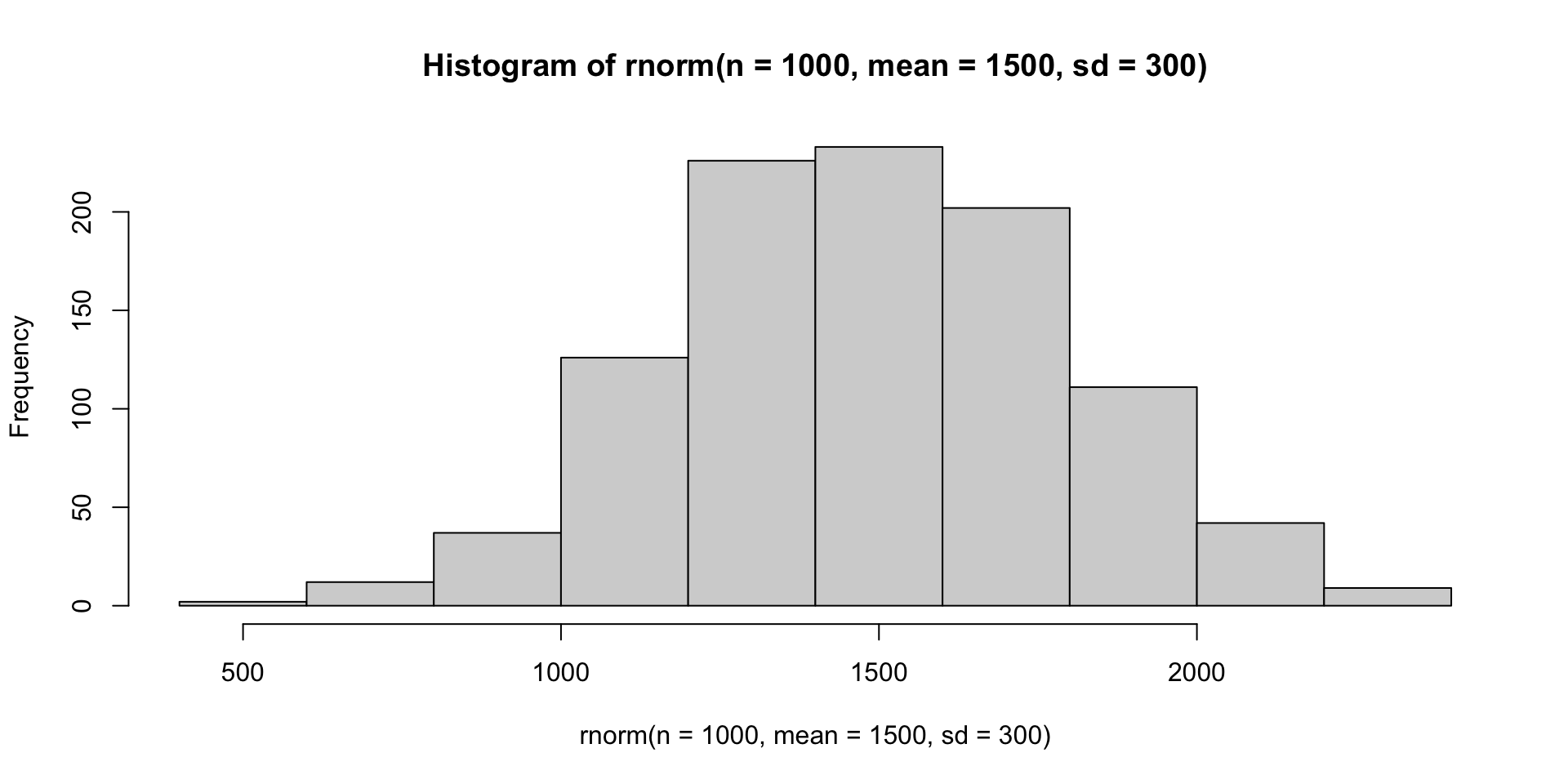
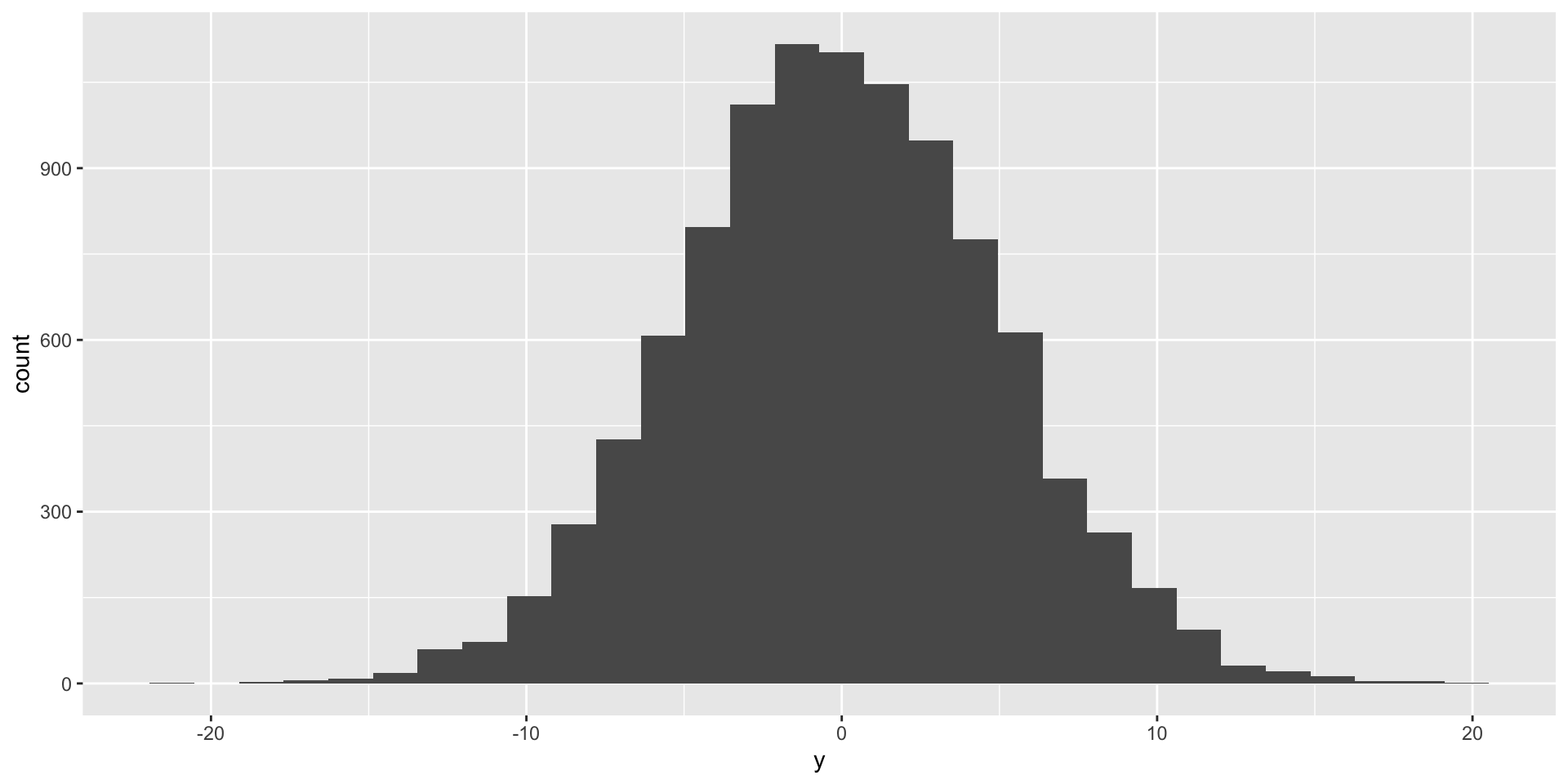
We can use rnorm() function to generate normal distribution data.

Code

rnorm(n = 100, mean = 0, sd = 1) |> # generate 100 data with mean 0 and standard deviation 1
  head() # show the first 6 data

[1]  0.9080765 -0.4112792  1.9168873  0.4132226 -0.5789695 -0.3337815

The first argument is the number of data we want to generate.
The second argument is the mean of the data.
The third argument is the standard deviation of the data.
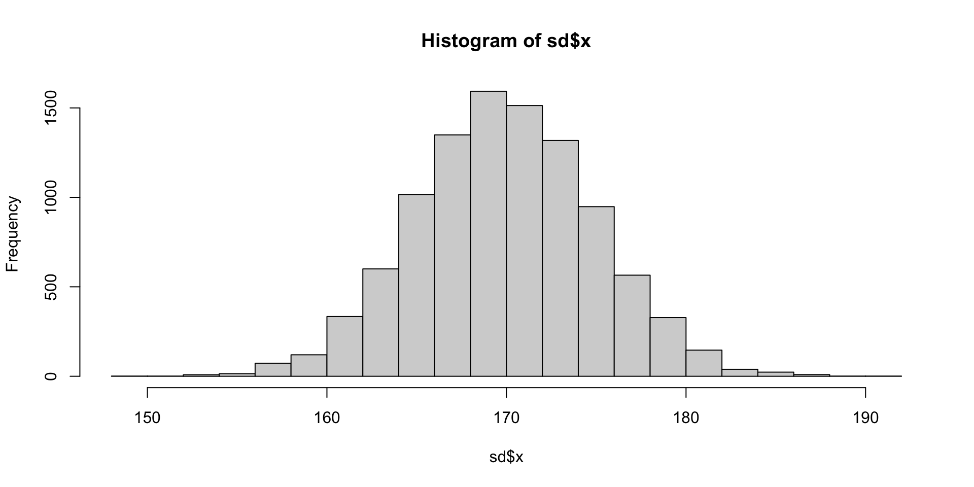
We can use hist() function to plot the data.

Code

rnorm(n = 1000, mean = 1500, sd = 300) |> # We can change the mean and standard deviation
  hist()

5 Standard normal distribution

During the period when there is no computer, people have to calculate the CDF by hand.
However, the PDF and CDF of standard normal distribution are quite complicated. It is hard to calculate, time-consuming, and easy to make mistakes.
To make it simple to calculate, we can standardize the normal distribution.

PDF of standard normal distribution

The pdf formula of standard normal distribution is:

\[ f(x) = {1 \over \sqrt{2\pi}} e^{-{x^2 \over 2}} \]

CDF of standard normal distribution

The cdf formula of standard normal distribution is:

\[ \Phi(x) = \int_{-\infty}^x f(x) dx = \int_{-\infty}^x {1 \over \sqrt{2\pi}} e^{-{x^2 \over 2}} dx \]

Compare to general normal distribution below:

\[ f(x) = {1 \over \sqrt{2\pi\sigma^2}} e^{-{(x-\mu)^2 \over 2\sigma^2}} \]

the mean and standard deviation of standard normal distribution are 0 and 1, respectively.

\[ \mu = 0 \] \[ \sigma = 1 \]

Standardize the normal distribution

We use an example to show how to standardize the normal distribution.

Code

# create a data with mean 170 and standard deviation 5
sd <- data.frame(
  x = rnorm(10000, 170, 5)
)

# Then plot the histogram of the data
hist(sd$x)

Code

# First subtract the mean of 170 from each data
sd |> 
  mutate(y = x - 170) |> 
  ggplot(aes(x = y)) +
  geom_histogram()# The mean of the data is 0 now

Code

# Second, divide each data by the standard deviation of 5
sd |> 
  mutate(y = x - 170,
         z = y / 5) |> 
  ggplot(aes(x = z, y = ..density..)) +
  geom_histogram() +
  geom_density()

Application of standard normal distribution

We can use standard normal distribution to compare two data with different mean and standard deviation.
For example, we have two data of exam scores, a is 2000 and b is 89 with mean 1500 and 75, and standard deviation 300 and 5, respectively. We want to know which score is better.
We can standardize the two data first, then compare their z scores.

Code

a <- (2000 - 1500) / 300
b <- (89 - 75) / 5

cat ("a = ", a, "\n")

a =  1.666667

Code

cat ("b = ", b, "\n")

b =  2.8

We can see that the z score of 2000 is 1.67, and the z score of 89 is 2.8. So the score of 89 is better than the score of 2000.
We can also use pnorm() function to calculate the probability of the two scores

Code

pnorm(q = 2000, mean = 1500, sd = 300)

[1] 0.9522096

Code

pnorm(q = 89, mean = 75, sd = 5)

[1] 0.9974449

2000 exceeds about 95.2% people, while 89 exceeds about 99.7% people. So 89 performs better than 2000.

6 Homework

Suppose the heights of students in a school follow a normal distribution with a mean of 65 inches and a standard deviation of 4 inches.

Determine the probability that a randomly selected student has a height higher than 69 inches (\(P(height > 69) = ?\)) without resorting to the Z-score table. Consider using the 68-95-99.7 rule, which provides approximate probabilities based on standard deviations in a normal distribution.
What is the probability that a randomly selected student is shorter than 71 inches (\(P(height<71)=?\))
Find the probability that a student is between 60 inches and 70 inches tall (\(P(60<height<70)=?\)).
Calculate the Z-score for a student who is 68 inches tall (\(Z=?\)).
Determine the height that corresponds to the 80th percentile (\(P(height<?)=0.8\)).
Imagine a country that uses cm scale to measure height. In a school within this country, student heights conform to a normal distribution with an average of 170 cm and a standard deviation of 6 cm. Given that a student from this school measures 178 cm in this system, how does this height compare in percentile to a student from the previous example, who measured 72 inches? Which student occupies the higher percentile rank in their school?

Thank you!