R programming for beginners (GV900)

Lesson 10: Central Limit Theorem

Reddy Lee

Saturday, January 13, 2024

Video of Lesson 10

1 Setup

In last lesson, we learned how to use normal distribution to solve problems. In this lesson, we will learn the Central Limit Theorem.

First, load the packages we will use in this lesson.

library(tidyverse)

2 Central limit theorem

• The Central Limit Theorem (CLT) states that the distribution of the average of a large number of independent, identically distributed (iid) variables will be approximately normal, regardless of the underlying distribution.

• We use an example of chi-square distribution to show CLT.

3 Chi-square distribution

• Chi-square distribution is a right-skewed distribution. It is used to test the goodness of fit of a model. It is also used to test the independence of two variables. We will learn more about it in the future lesson. Here we just use it as an example to show CLT.

tibble(
  sample = 1:10000,
  value = rchisq(10000, df = 5)
) |> 
  ggplot(aes(x = value, y = ..density..)) +
  geom_histogram(bins = 30, color = "white", fill = "steelblue") +
  geom_density(color = "purple", size = 1)

# Step 1, create a chi-square distribution 
chidata <- tibble(
  sample = 1:100,
  value = rchisq(100, df = 3)
)

hist(chidata$value)

# Step 2: repeat it
chidata2 <- tibble(
  sample = 1:100,
  value = rchisq(100, df = 3)
)

hist(chidata2$value)

# Step 3: repeat it again
chidata3 <- tibble(
  sample = 1:100,
  value = rchisq(100, df = 3)
)

hist(chidata3$value)

tibble(
  sample = 1:10000, # sample size = 10000
  value = rchisq(10000, df = 3)
) |> 
  ggplot(aes(x = value, y = ..density..)) +
  geom_histogram(bins = 30, color = "white", fill = "steelblue") +
  geom_density(color = "purple", size = 1) 

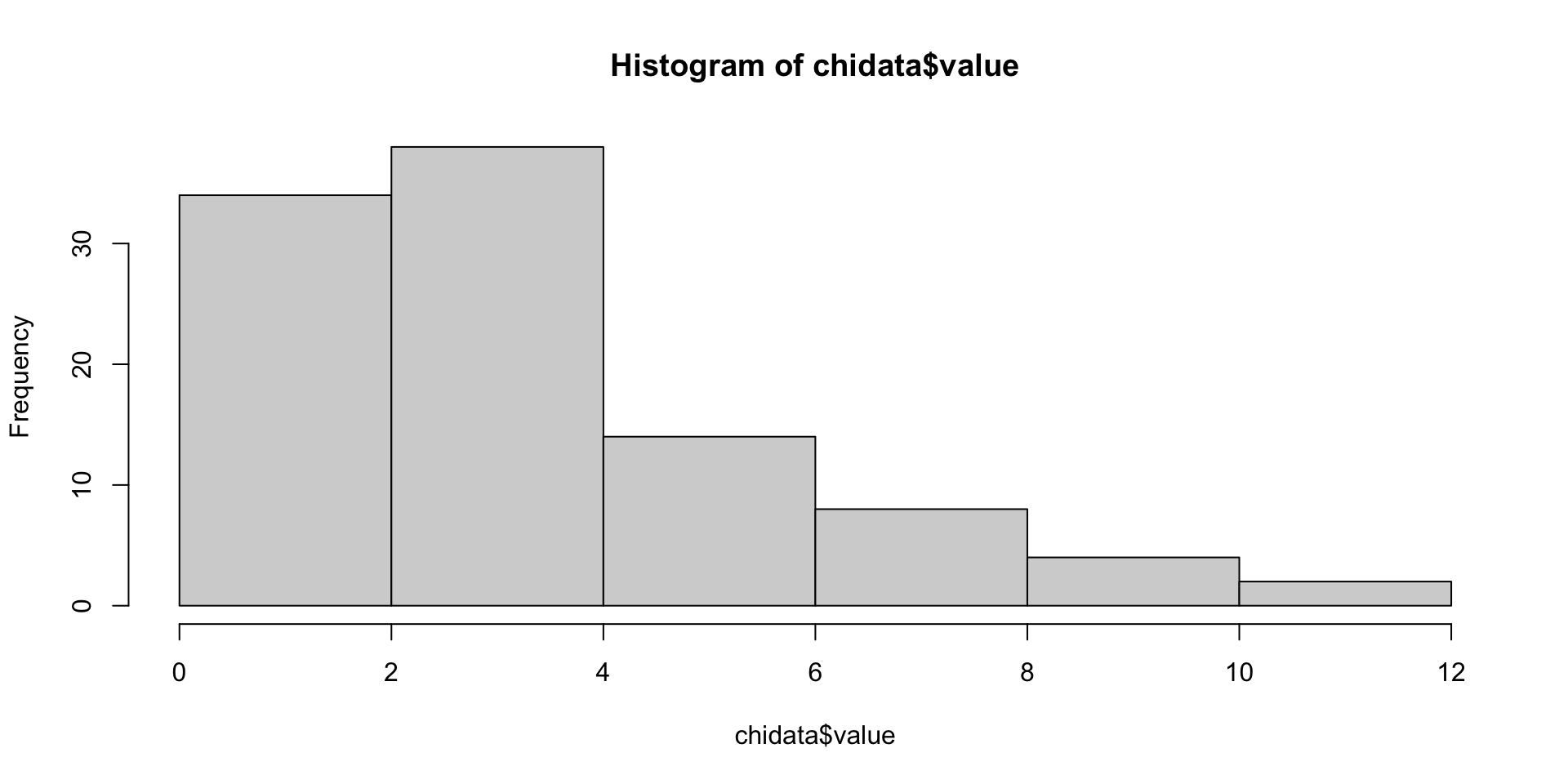
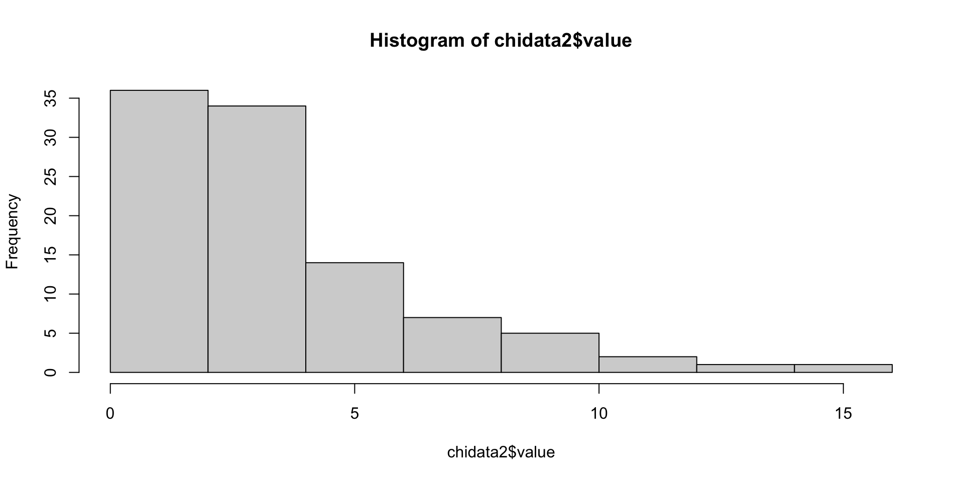
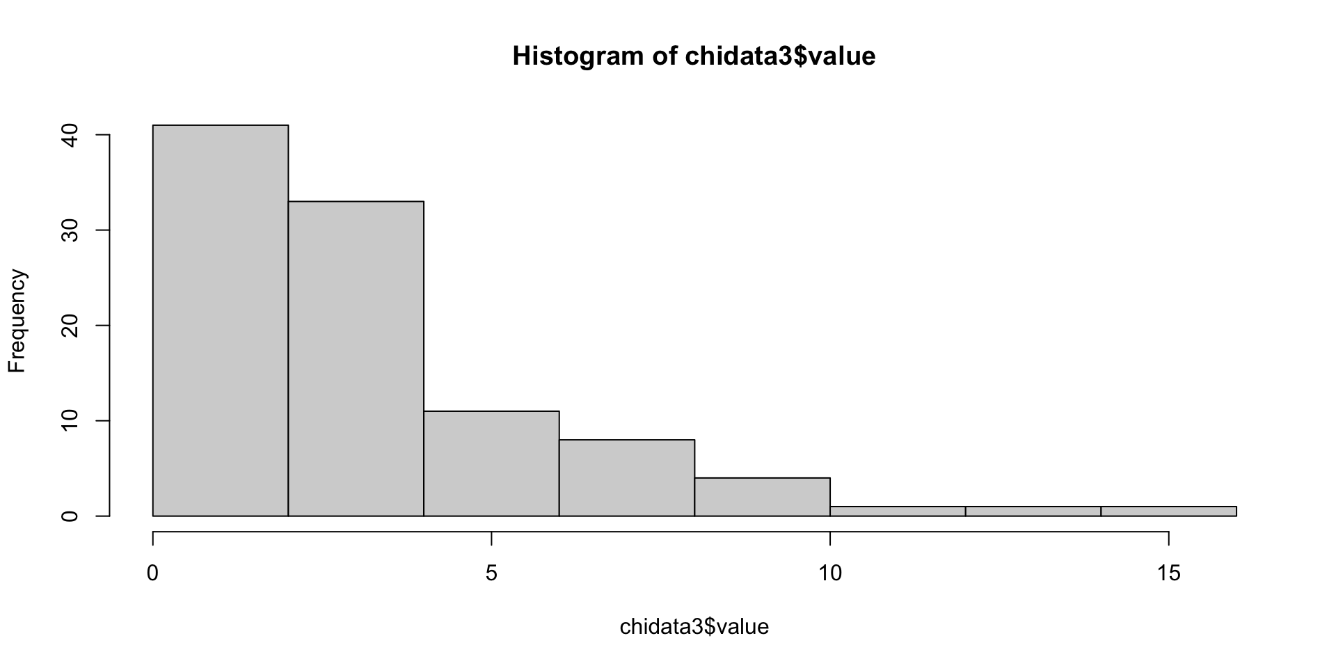
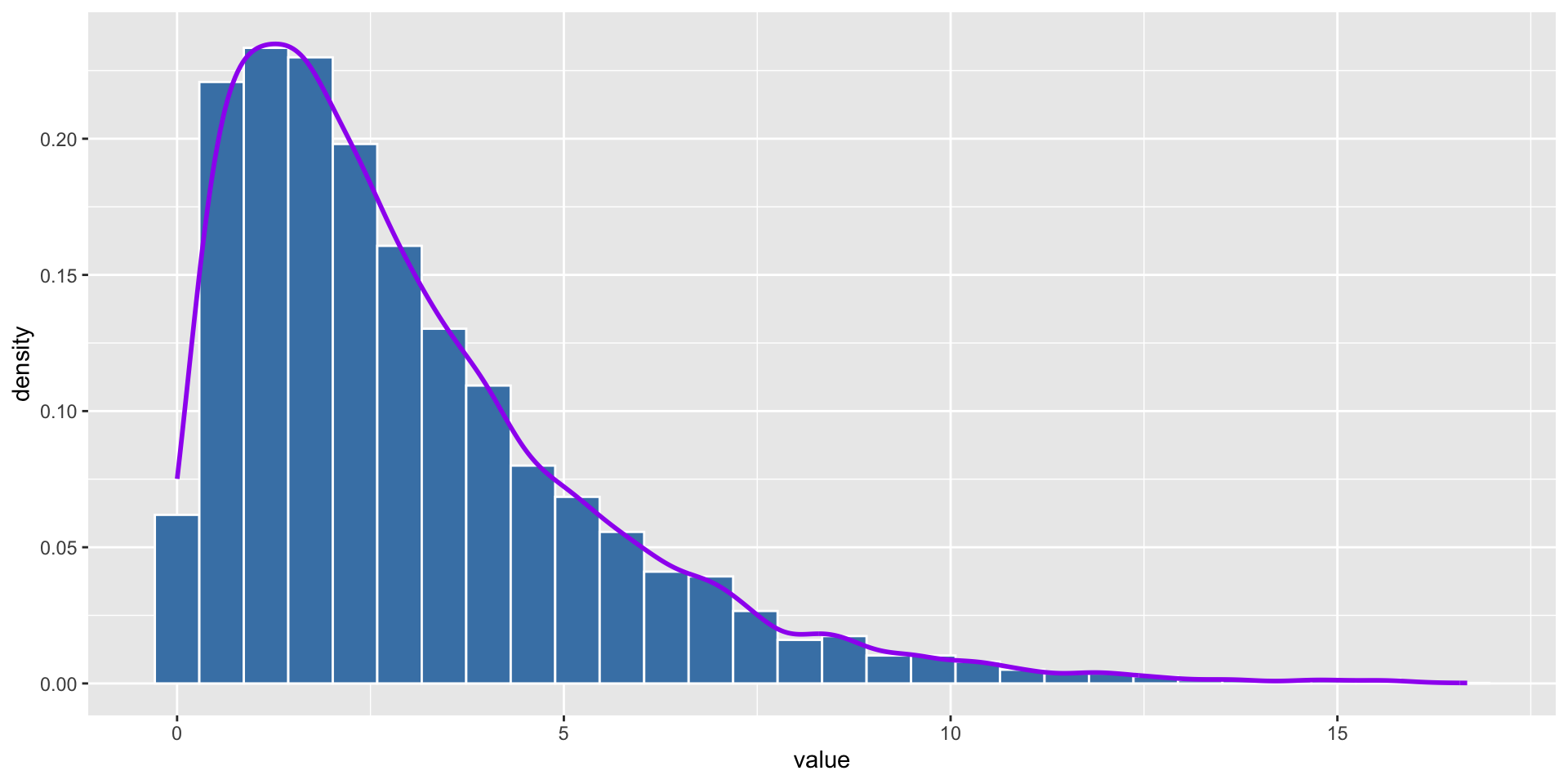
• We can see that the distributions of the three samples are chi-square distributions which are right-skewed. They are not normal distribution.

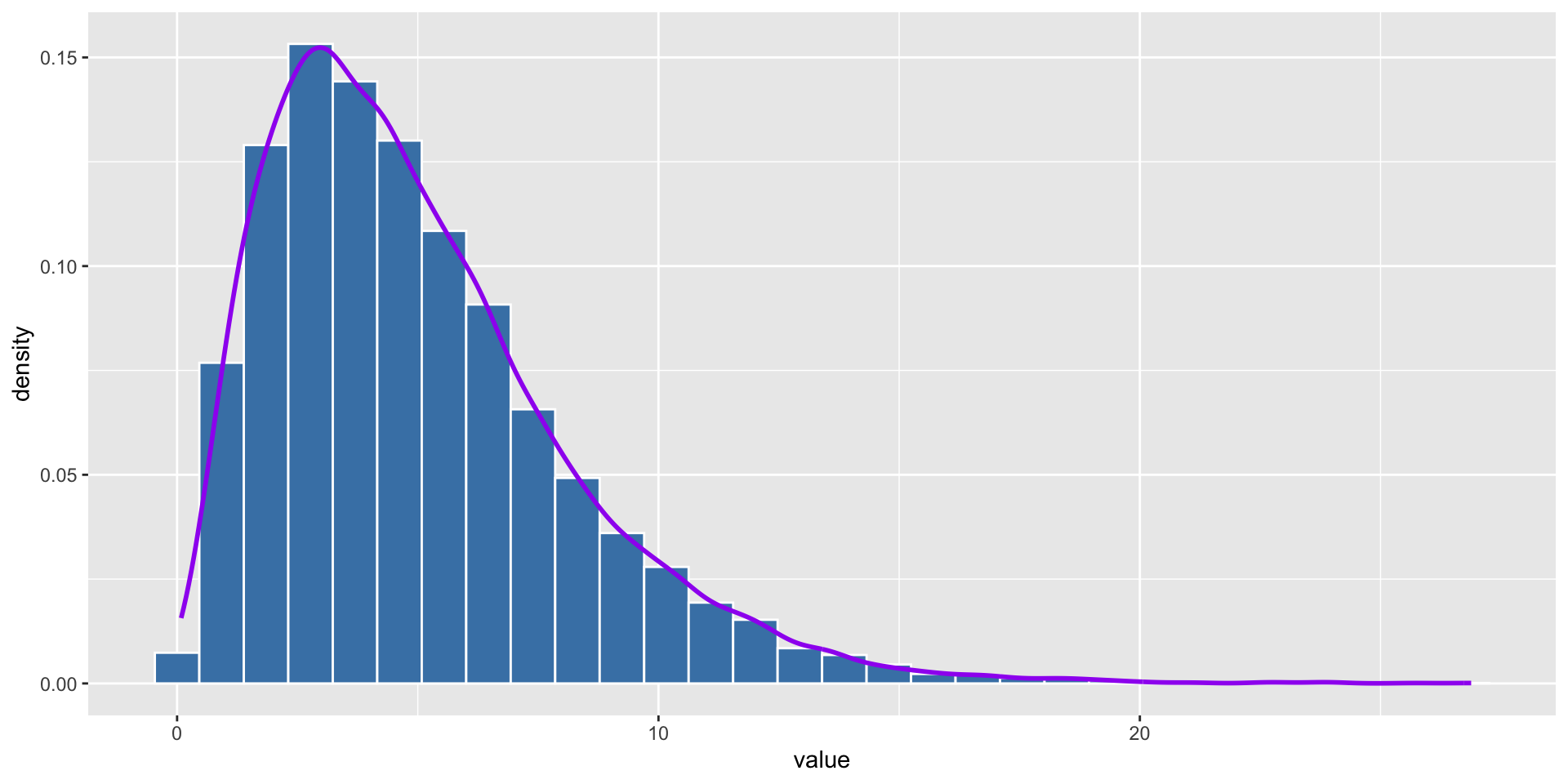
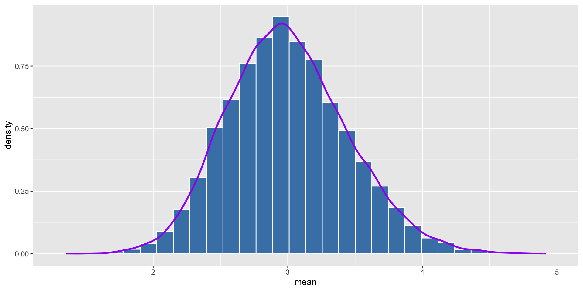
• Let’s see what happens after we repeat it 10000 times with sample size of 10.

# Step 4, Repeat the experiment 10000 times, with sample size of 30, calculate the average of each sample
tibble(
  experiment = 1:10000,
  mean = replicate(10000, mean(rchisq(10, df = 3))) 
) |> 
  ggplot(aes(x = mean, y = ..density..)) +
  geom_histogram(bins = 30, color = "white", fill = "steelblue") +
  geom_density(color = "purple", size = 1)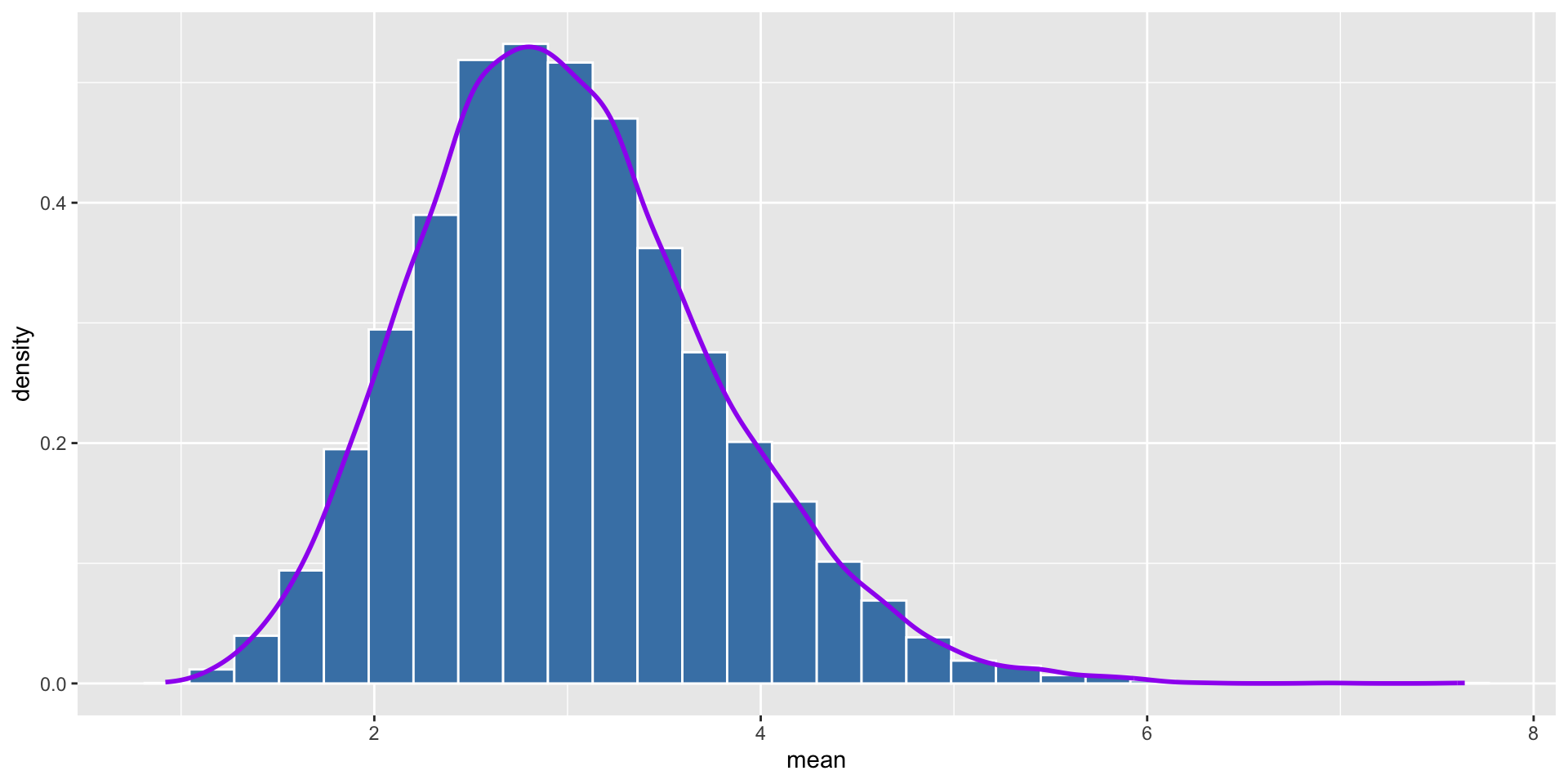

• We can see that the distribution of the average of each sample is normal distribution.

• Let’s see what happens if we repeat it 10000 times with the sample size of 5.

# Step 5, sample size = 5
tibble(
  experiment = 1:10000,
  mean = replicate(10000, mean(rchisq(5, df = 3))) 
) |> 
  ggplot(aes(x = mean, y = ..density..)) +
  geom_histogram(bins = 30, color = "white", fill = "steelblue") +
  geom_density(color = "purple", size = 1)

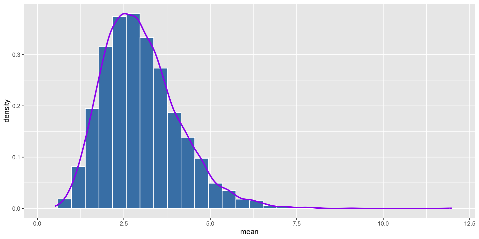
• Let’s try with the sample size of 10.

# Step 6, sample size = 10
tibble(
  experiment = 1:10000,
  mean = replicate(10000, mean(rchisq(10, df = 3))) 
) |> 
  ggplot(aes(x = mean, y = ..density..)) +
  geom_histogram(bins = 30, color = "white", fill = "steelblue") +
  geom_density(color = "purple", size = 1)

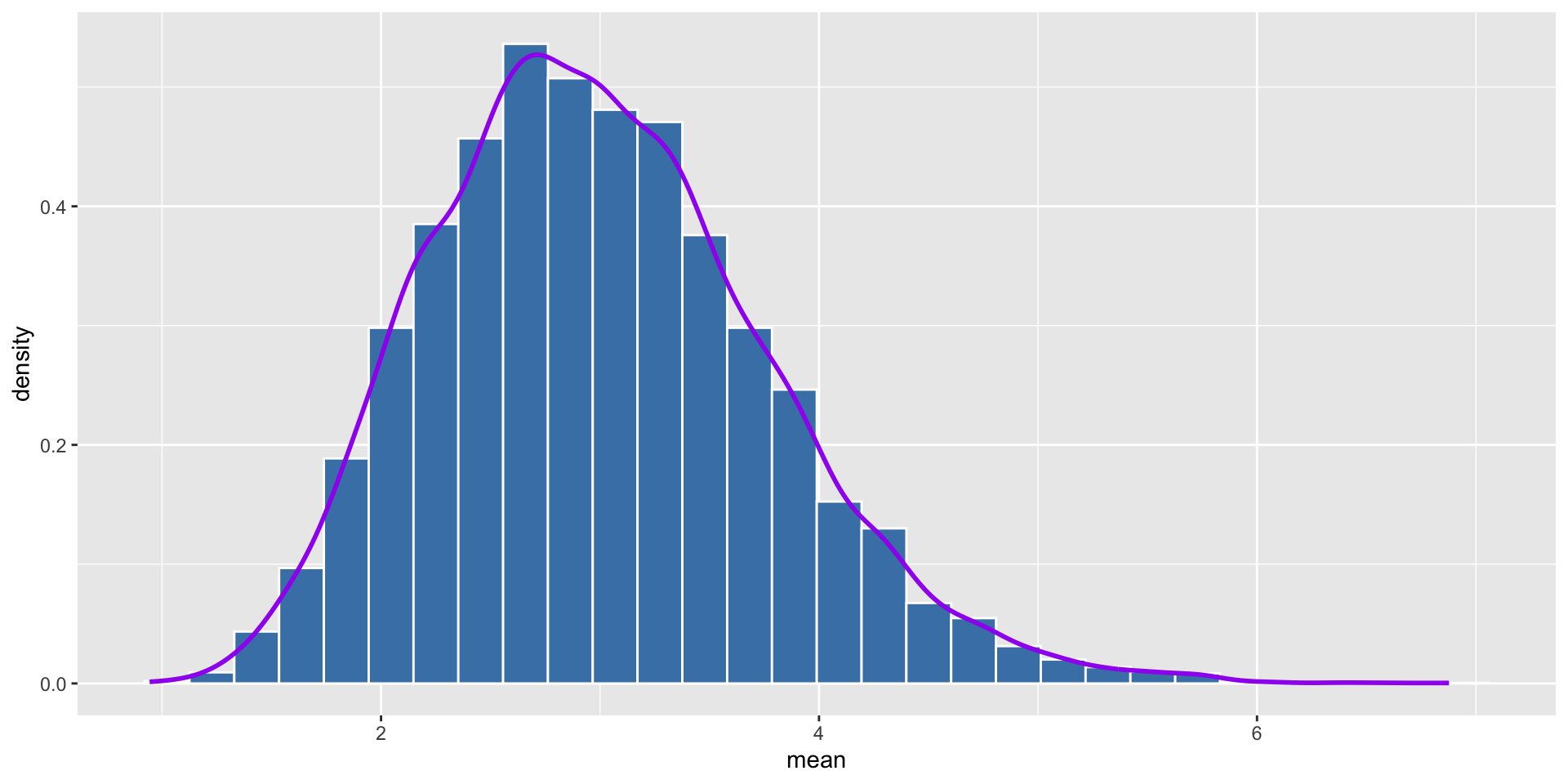
• With sample size of 30

# Step 7, sample size = 30
tibble(
  experiment = 1:10000,
  mean = replicate(10000, mean(rchisq(30, df = 3))) 
) |> 
  ggplot(aes(x = mean, y = ..density..)) +
  geom_histogram(bins = 30, color = "white", fill = "steelblue") +
  geom_density(color = "purple", size = 1)

• With sample size of 100

# Step 8, sample size = 100
tibble(
  experiment = 1:10000,
  mean = replicate(10000, mean(rchisq(100, df = 3))) 
) |> 
  ggplot(aes(x = mean, y = ..density..)) +
  geom_histogram(bins = 30, color = "white", fill = "steelblue") +
  geom_density(color = "purple", size = 1)

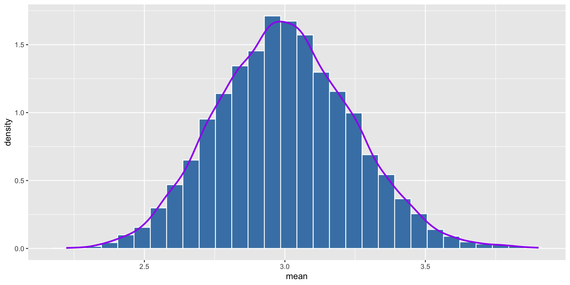
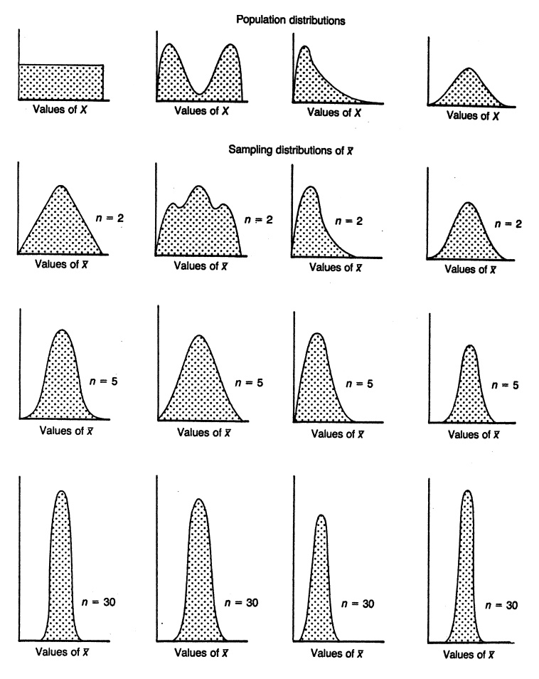
• We can see that the distribution of the average of each sample is more like normal distribution as the sample size increases. Normally, we say that the sample size is large enough when it is greater than 30.

• If we use different distributions, the distribution of the average of each sample (sampling distribution) will be normal distribution as well.

Thank you!