R programming for beginners (GV900)

Lesson 11: Standard Deviation and Standard Error

Sunday, January 14, 2024

Video of Lesson 11

1 Setup

In this lesson, we will learn the standard deviation and the standard error.

First, load the packages we will use in this lesson.

Code

library(tidyverse)
library(carData)

2 Standard Deviation

Standard Deviation

The standard deviation is a measure of how spread out the values are from the mean.

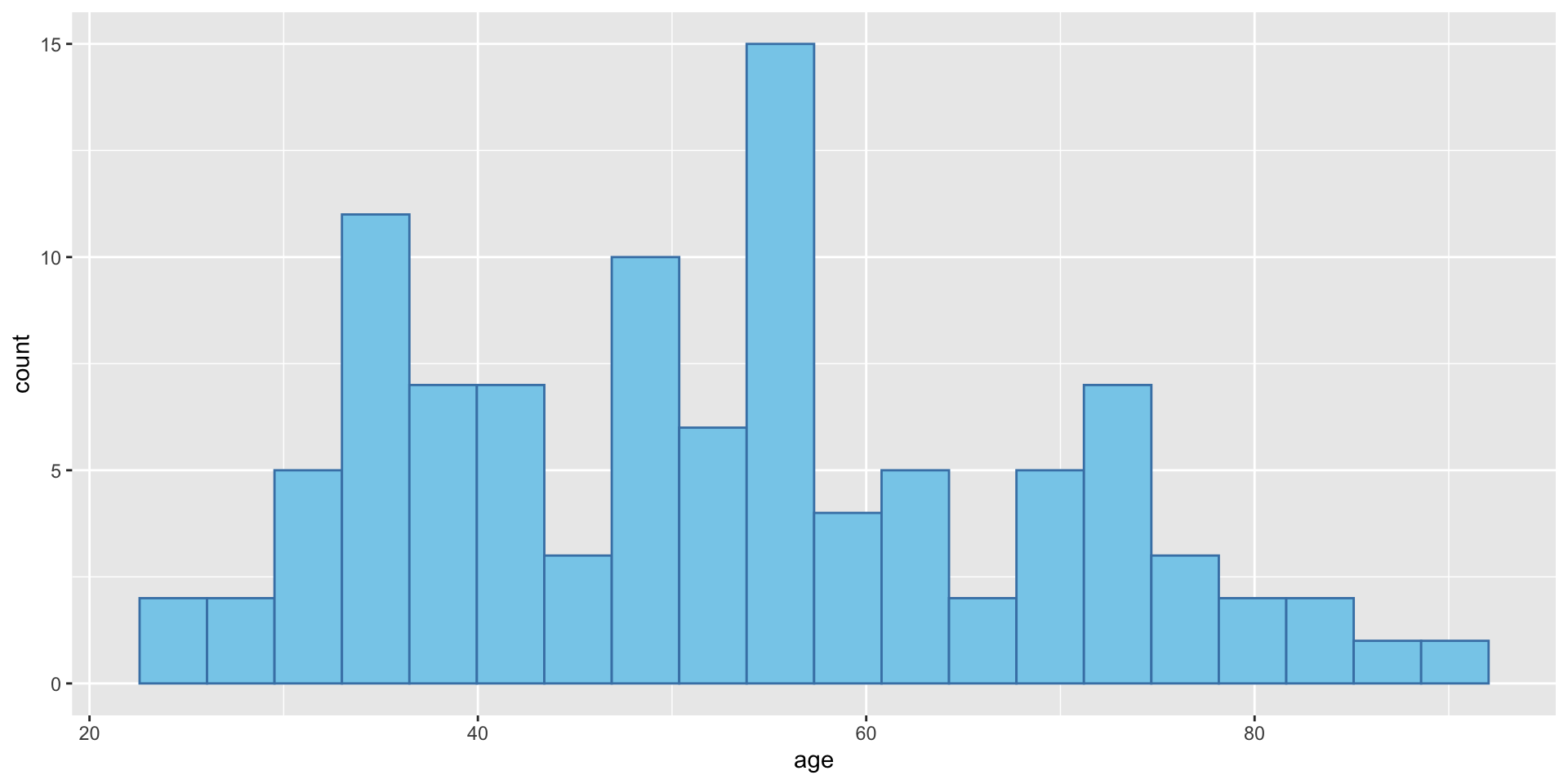
First let us calculate the standard deviation of the age variable in the BEPS dataset by hand.

\[\begin{aligned} Var &= {\sum_{i=1}^n(y_i-\bar{y})^2 \over n-1} \\ \\ sd &= \sqrt{Var} \\ \\ &= \sqrt{{\sum_{i=1}^n(y_i-\bar{y})^2 \over n-1}} \end{aligned}\]

First let us calculate the variance of the age variable in the BEPS dataset by hand.

Code

# view(BEPS)
BEPS |> 
  select(age) |> 
  mutate(age_mean = mean(age)) |> 
  mutate(age_diff = age - age_mean) |> 
  mutate(age_diff_sq = age_diff^2) |>
  summarise(Sum_square = sum(age_diff_sq),
            n = n(),
            Var = sum(age_diff_sq)/(n()-1),
            sd = sqrt(Var))

  Sum_square    n      Var       sd
1   376187.3 1525 246.8421 15.71121

With R, we can use the sd() function to calculate the standard deviation easily.

Code

BEPS |> 
  summarise(Var = var(age),
              sd = sd(age))

       Var       sd
1 246.8421 15.71121

3 Degrees of Freedom

Why we use n()-1 instead of n() in the variance formula? When we calculate the variance, we use the mean of the sample, which itself is estimated from the sample. For example, if we have a sample of 10 numbers, the mean of the 10 numbers is decided by the 10 numbers. But if we know the mean of the 10 numbers, you are free to choose the 10 numbers. Actually, not 10 numbers. When you’ve chosen 9 numbers, you will find that you cannot freely choose the 10th number if you wish get the pre-decided mean. Therefore, we only have 9 degrees of freedom in this case.

Degrees of Freedom

The degrees of freedom is the number of independent observations in a sample minus the number of population parameters that must be estimated from sample data.

4 Standard Error

Standard Error

The standard error is the standard deviation of the sampling distribution of a statistic.

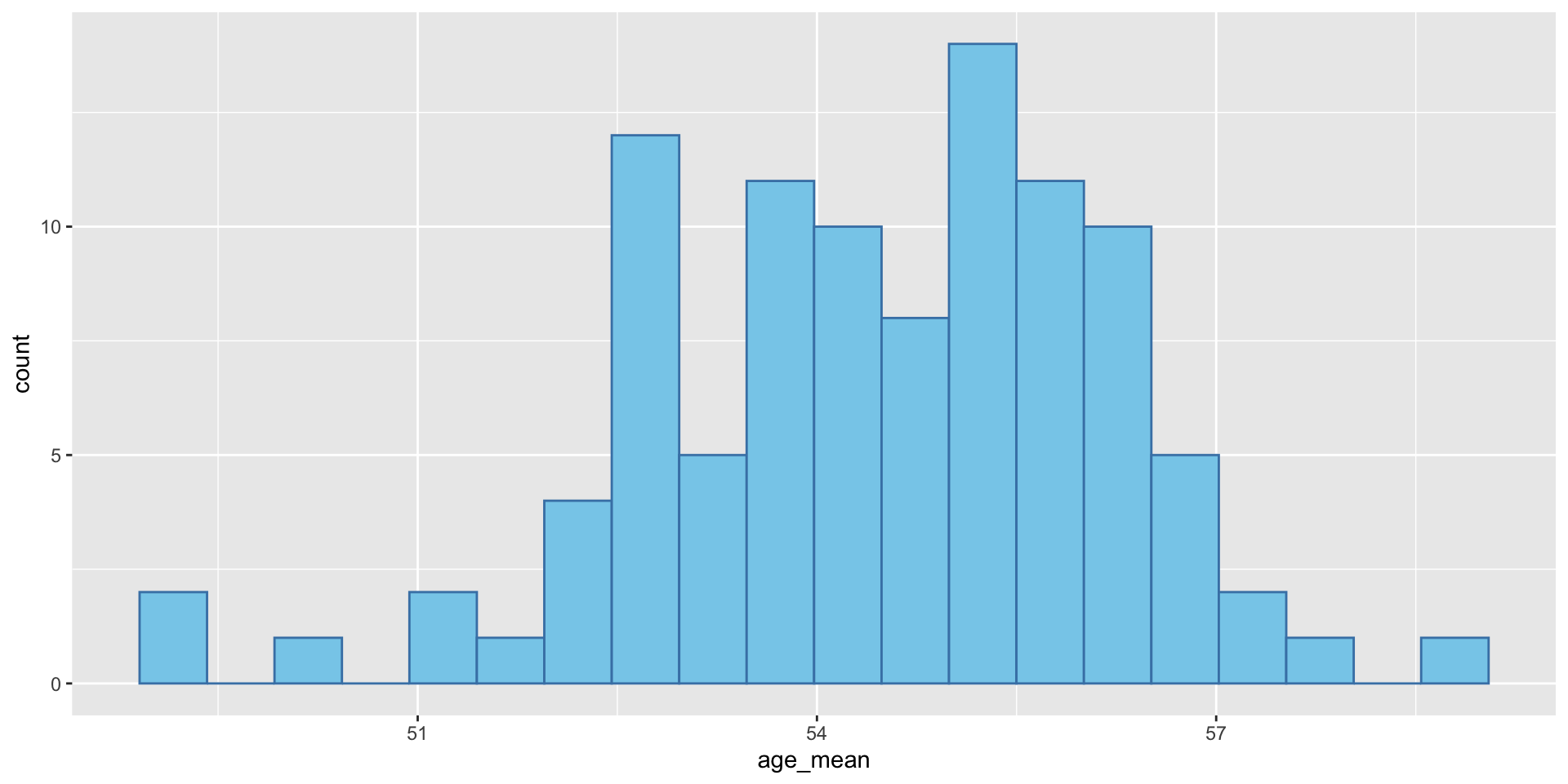
First let us calculate the standard error of the mean of the age variable in the BEPS dataset by hand.

Code

# one sample
BEPS |> 
  select(age) |>
  slice_sample(n = 100) |>
  summarise(age_mean = mean(age))

  age_mean
1    52.08

Code

# 100 samples
# Don't worry if you don't understand this code. We will learn the for loop function in the future lessons.
age_mean <- numeric(100)

# Loop to generate 100 age_mean values
for (i in 1:100) {
  age_mean[i] <- BEPS %>%
    select(age) %>%
    slice_sample(n = 100, replace = TRUE) %>%
    summarise(age_mean = mean(age)) %>%
    pull(age_mean)
}

# Display the first few age_mean values
age_means <- data.frame(sample = 1: 100,
                        age_mean)

Code

# Now we can calculate the standard deviation of the 100 age_mean values with the sd() function.
sd(age_means$age_mean)

[1] 1.745488

However, we don’t need to do this by hand. We don’t need to create 100 samples either. Even it is possible to survey 100 samples, it is time-consuming and costly. There is a easier way to calculate the standard error of the mean.

\[\begin{aligned} se &= {sd \over \sqrt n} \\ \\ &= {\sqrt{{\sum_{i=1}^n(y_i-\bar{y})^2 \over n-1}} \over \sqrt n} \end{aligned}\]

Code

# We use one sample of 100 observations to calculate the standard error of the mean.

BEPS |> 
  select(age) |>
  slice_sample(n = 100) |>
  summarise(age_mean = mean(age),
            sd = sd(age),
            se = sd/sqrt(n()))

  age_mean       sd       se
1    53.61 15.97403 1.597403

We can see that the se calculated by \(sd \over \sqrt(n)\) is very close to the sd of the 100 age_mean values we calculated before.
We can easily notice that the standard error of the mean is dependent on the sample size (\(n\)). The larger the sample size, the smaller the standard error of the mean.
However, if we increase the sample times but keep the sample size unchanged, the standard error of the mean will not change significantly.

Code

# histogram of one sample of 100 observations
BEPS |> 
  select(age) |>
  slice_sample(n = 100) |> 
  ggplot(aes(x = age)) +
  geom_histogram(bins = 20, fill = "skyblue", color = "steelblue")

Code

# histogram of the 100 age_mean values
age_means |> 
  ggplot(aes(x = age_mean)) +
  geom_histogram(bins = 20, fill = "skyblue", color = "steelblue")

5 Recap

In this lesson, we learned the standard deviation and the standard error.
- The standard deviation is a measure of how spread out the values are from the mean.
- The standard error is the standard deviation of the sampling distribution of a statistic.
- The standard error of the mean is dependent on the sample size (\(n\)). The larger the sample size, the smaller the standard error of the mean.
In the following lessons, we will use sampling distribution and the standard error to calculate the confidence interval of the mean, and do hypothesis testing.

Thank you!