R programming for beginners (GV900)

Lesson 13: Proportion Z test

Reddy Lee

Monday, January 15, 2024

Video of Lesson 13

1 Setup

In this lesson, we will learn the proportion Z test.

First, load the packages we will use in this lesson.

library(tidyverse)
library(janitor)
library(openintro)
library(carData)

2 Proportion Z test

Proportion Z-test

Proportion Z test is a hypothesis test for the population proportion. It is used to test categorical data.

• Let’s take a look at the distribution of the variable gender in the BEPS dataset of carData.

#View(BEPS)

# summary(BEPS$gender) # table(BEPS$gender)
# summary(BEPS$age)
BEPS |> 
  tabyl(gender) # You need to load the janitor package

 gender   n  percent
 female 812 0.532459
   male 713 0.467541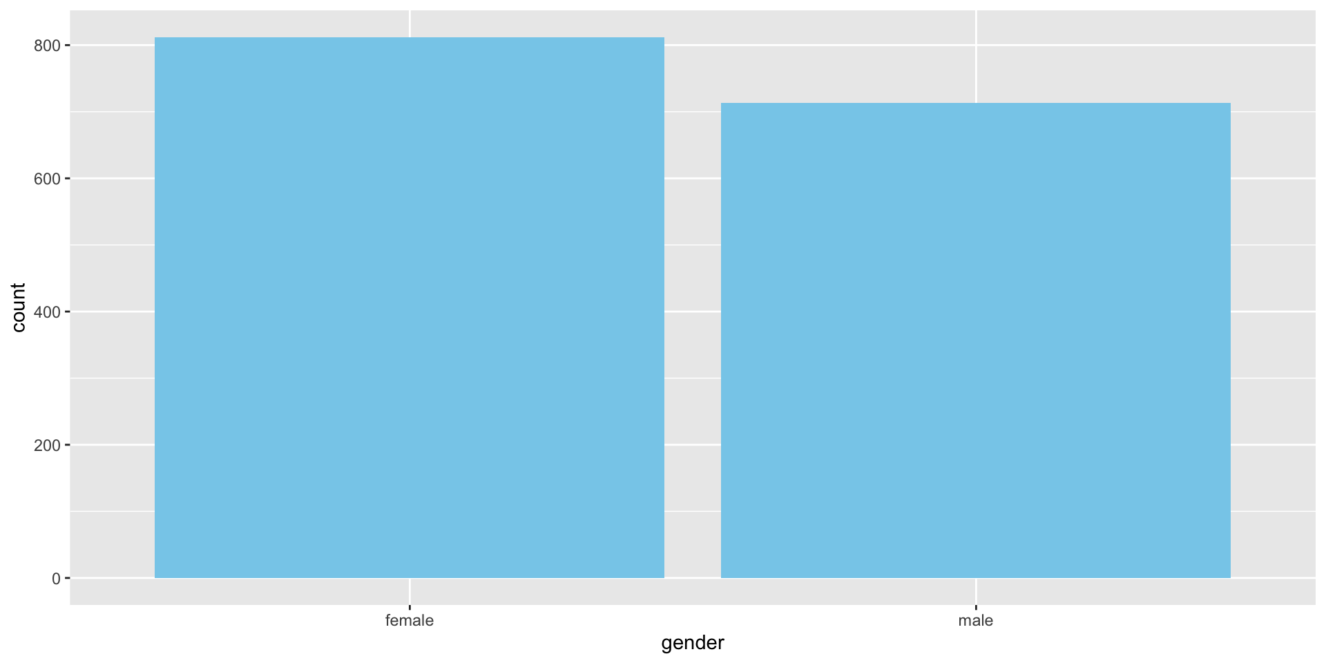

# Visualize the gender variable
BEPS |> 
  ggplot(aes(x = gender)) +
  geom_bar(fill = "skyblue")

3 One-proportion Z test

• Hypothesis test for one proportion

• The null hypothesis (\(H0\)) is that the population proportion of female is equal to \(0.5\).

• The alternative hypothesis (\(H1\)) is that the population proportion of female is not equal to \(0.5\).

\[\begin{aligned} Z &= {(p_1 - p_0)\over se } \\ \\ &={(p_1 - p_0)\over {\sigma\over \sqrt n} } \\ \\ &= {(p_1 - p_0)\over \sqrt {p_0 (1- p_0) \over n} } \end{aligned}\]

• Examples

• Here Z is the test statistic, \(p_1\) is the sample proportion, \(p_0\) is the hypothesized proportion, and \(n\) is the sample size. \(se\) is the standard error of the sample proportion, and \(\sigma\) is the standard deviation of the sampling distribution of the sample proportion.

prop.test(x = 812, n = 1525, p = 0.5, alternative = "two.sided")

    1-sample proportions test with continuity correction

data:  812 out of 1525, null probability 0.5
X-squared = 6.2977, df = 1, p-value = 0.01209
alternative hypothesis: true p is not equal to 0.5
95 percent confidence interval:
 0.5070389 0.5577139
sample estimates:
       p 
0.532459 

• The first argument is the number of female, the second argument is the sample size, and the third argument is the hypothesized proportion. The fourth argument is the alternative hypothesis. The default alternative hypothesis is that the population proportion is not equal to the hypothesized proportion. And the default significance level is 0.05.

• In this significance level, we reject the null hypothesis because the p-value is less than the significance level 0.05. And the confidence interval does not contain the hypothesized proportion 0.5.

• We can also change the significance level to \(0.01\) by adding the argument conf.level = 0.99.

prop.test(x = 812, n = 1525, p = 0.5, alternative = "two.sided", conf.level = 0.99)

    1-sample proportions test with continuity correction

data:  812 out of 1525, null probability 0.5
X-squared = 6.2977, df = 1, p-value = 0.01209
alternative hypothesis: true p is not equal to 0.5
99 percent confidence interval:
 0.4991511 0.5654829
sample estimates:
       p 
0.532459 

• In the 0.01 significance level, we fail to reject the null hypothesis because the p-value is greater than the significance level 0.01. And the confidence interval contains the hypothesized proportion 0.5.

• We can also change the alternative hypothesis to “less” or “greater” by adding the argument alternative = "less" or alternative = "greater".

• Since the sample proportion is greater than the hypothesized proportion, we can use the alternative hypothesis “greater”.

prop.test(x = 812, n = 1525, p = 0.5, alternative = "greater")

    1-sample proportions test with continuity correction

data:  812 out of 1525, null probability 0.5
X-squared = 6.2977, df = 1, p-value = 0.006045
alternative hypothesis: true p is greater than 0.5
95 percent confidence interval:
 0.5110761 1.0000000
sample estimates:
       p 
0.532459 

• In the 0.05 significance level, we reject the null hypothesis because the p-value is less than the significance level 0.05. And the confidence interval does not contain the hypothesized proportion 0.5.

• We can also change the hypothesized proportion to 0.6 by adding the argument p = 0.6. The null hypothesis is that the population proportion of female is equal to \(0.6\).

prop.test(x = 812, n = 1525, p = 0.6, alternative = "two.sided")

    1-sample proportions test with continuity correction

data:  812 out of 1525, null probability 0.6
X-squared = 28.706, df = 1, p-value = 8.426e-08
alternative hypothesis: true p is not equal to 0.6
95 percent confidence interval:
 0.5070389 0.5577139
sample estimates:
       p 
0.532459 

• In the 0.05 significance level, we reject the null hypothesis because the p-value is less than the significance level 0.05. And the confidence interval does not contains the hypothesized proportion 0.6.

4 Two-proportion Z test

Two-proportion Z test

Two-proportion Z test is a hypothesis test for the difference between two population proportions. It is also used to test categorical data.

• Hypotheses:
  • Null Hypothesis (\(H0\)): The proportions in the two groups are equal.
  • Alternative Hypothesis (\(H1\)): The proportions in the two groups are not equal.

\[\begin{aligned} Z &= {(p_1 - p_2)\over \sqrt{p(1-p)({1\over n_1} + {1\over n_2})}} \end{aligned}\]

• Here Z is the test statistic, \(p_1\) is the sample proportion of group 1, \(p_2\) is the sample proportion of group 2, \(p\) is the pooled proportion, \(n_1\) is the sample size of group 1, and \(n_2\) is the sample size of group 2.

\[\begin{aligned} p ={ n_1 p_1 + n_2 p_2 \over n_1 + n_2} \end{aligned}\]

• Examples

• Let’s say we have another sample which is from the voting data of USA, the gender proportion is \(female = 3120\) while \(male = 2880\), so the total sample of USA is 6000

prop.test(x = c(812, 3120), n = c(1525, 6000))

    2-sample test for equality of proportions with continuity correction

data:  c(812, 3120) out of c(1525, 6000)
X-squared = 0.70741, df = 1, p-value = 0.4003
alternative hypothesis: two.sided
95 percent confidence interval:
 -0.01600389  0.04092192
sample estimates:
  prop 1   prop 2 
0.532459 0.520000 

• The first argument is the number of successes in group 1 and group 2, the second argument is the sample size of group 1 and group 2, and the alternative hypothesis and the default significance level is “two.sided” and “0.05”.

• In the 0.05 significance level, we fail to reject the null hypothesis because the p-value is greater than the significance level 0.05. And the confidence interval contain 0.

5 Recap

• In this lesson, we learned the one-proportion and two-proportion Z test.

• The one-proportion Z test is a hypothesis test for one population proportion. It is used to test categorical data.

• The two-proportion Z test is a hypothesis test for the difference between two population proportions.

• In next lesson, we will learn the t-test.

Thank you!