R programming for beginners (GV900)

Lesson 14: T distribution & T test

Reddy Lee

Wednesday, January 17, 2024

Video of Lesson 14

1 Outline

• In this lesson, we will learn:

  • T distribution

  • T test

• First, load the packages we will use in this lesson.

library(tidyverse)
library(openintro)
library(gapminder)

2 t distribution (Student’s distribution)

Question?

• Q: Why we need t distribution since we already have normal distribution?
• A: Because we don’t know the standard deviation of the population, and the sample size is small.

• The t distribution is a family of distributions that look similar to the normal distribution but have heavier tails.

• The t distribution is used for inference on the mean when the population standard deviation is unknown.

• The t distribution is centred at zero and has a parameter called degrees of freedom.

• The degrees of freedom is equal to the sample size minus one.

• As the degrees of freedom increases, the t distribution approaches the normal distribution.

normTail(m = 0, s = 1, df = 5, M = c(-2.5,2.5), border  = "skyblue", col = NULL,
         xLab = "symbol", axes = 3)

normTail(m = 0, s = 1, df = 3, M = c(-2.5,2.5), border = "blue",
         xLab = "symbol", axes = 3, add = TRUE, col = NULL)

normTail(m = 0, s = 1, df = 30, M = c(-2.5,2.5), border = "purple",
         xLab = "symbol", axes = 3, add = TRUE, col = NULL)

normTail(m = 0, s = 1, M = c(-2.5,2.5), border = "red",
         xLab = "symbol", axes = 3, add = TRUE, col = NULL)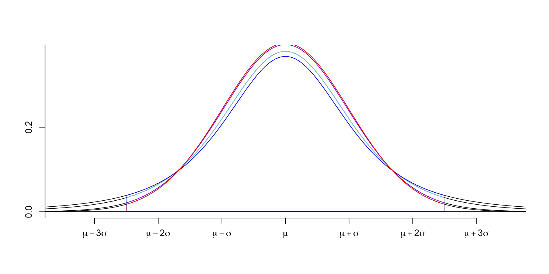

• As the long tail of the t distribution, the t distribution has more probability in the tails than the normal distribution.

• So, to cover the same area under the curve, the t distribution has a wider spread than the normal distribution.

• And we use a larger critical value for the t distribution than the normal distribution.

• Compare the formulas of confidence interval for the mean of normal distribution and t distribution.

\[\bar{x} \pm Z_{\alpha / 2} \frac{s}{\sqrt{n}}\]

\[ \bar{x} \pm t_{n-1, \alpha / 2} \frac{s}{\sqrt{n}} \]

where \({Z_{\alpha / 2}}\) is the critical value of the normal distribution and \(t_{n-1, \alpha / 2}\) is the critical value of the t distribution.

3 One sample t test

• The one sample t test is used to compare the mean of a single sample to a known value or any value we choose to test.

• For example, we might want to know if the average height of a group of people is different from 170 cm.

• The null hypothesis is that the mean is equal to 170 cm, and the alternative hypothesis is that the mean is not equal to 170 cm.

• The test statistic is calculated as:

\[t = \frac{\bar{x} - \mu}{s/\sqrt{n}}\]

where \(\bar{x}\) is the sample mean, \(\mu\) is the known value, \(s\) is the sample standard deviation, and \(n\) is the sample size.

• The test statistic follows a t distribution with \(n-1\) degrees of freedom.

• Example for one sample t test

gapminder |> 
  filter(year == 2007) |> 
  t.test(lifeExp ~ 1, mu = 70, data = _)

    One Sample t-test

data:  lifeExp
t = -2.9537, df = 141, p-value = 0.00368
alternative hypothesis: true mean is not equal to 70
95 percent confidence interval:
 65.00450 69.01034
sample estimates:
mean of x 
 67.00742 

• In this case, we reject the null hypothesis and conclude that the average life expectancy in 2007 is not equal to 70 years old.

4 Two sample t test

• The two sample t test is used to compare the means of two independent samples.

• The formula for the test statistic is:

\[t = \frac{\bar{x}_1 - \bar{x}_2}{\sqrt{\frac{s_1^2}{n_1} + \frac{s_2^2}{n_2}}}\]

where \(\bar{x}_1\) and \(\bar{x}_2\) are the sample means, \(s_1\) and \(s_2\) are the sample standard deviations, and \(n_1\) and \(n_2\) are the sample sizes.

gapminder |> 
  filter(year == 2007,
         continent  %in% c("Asia", "Africa")) |> 
  t.test(lifeExp ~ continent, data = _)

    Welch Two Sample t-test

data:  lifeExp by continent
t = -8.2715, df = 77.225, p-value = 2.991e-12
alternative hypothesis: true difference in means between group Africa and group Asia is not equal to 0
95 percent confidence interval:
 -19.75539 -12.08951
sample estimates:
mean in group Africa   mean in group Asia 
            54.80604             70.72848 

• In this case, we reject the null hypothesis and conclude that the average life expectancy in 2007 is not equal between Asia and Africa.

5 Paired t test

• The paired t test is used to compare the means of two dependent samples. It usually used in situations where the same sample is measured in different times or conditions.

• The formula for the test statistic is:

\[t = \frac{\bar{x}_d}{s_d/\sqrt{n}}\]

where \(\bar{x}_d\) is the sample mean of the differences, \(s_d\) is the sample standard deviation of the differences, and \(n\) is the sample size.

gapminder |> 
  filter(year %in% c(1952, 2007)) |> 
  t.test(lifeExp ~ year, paired = TRUE, data = _)

    Paired t-test

data:  lifeExp by year
t = -26.327, df = 141, p-value < 2.2e-16
alternative hypothesis: true mean difference is not equal to 0
95 percent confidence interval:
 -19.29766 -16.60194
sample estimates:
mean difference 
       -17.9498 

• In this case, we reject the null hypothesis and conclude that the average life expectancy in 2007 is not equal to 1952.

• This is equivalent to the following one-sample t test:

gapminder |> 
  filter(year  %in% c(1952, 2007)) |> # filter rows
  select(country, year, lifeExp) |> # select columns
  spread(year, lifeExp) |> # long to wide
  mutate(diff = `2007` - `1952`) |> # calculate the difference
  t.test(diff ~ 1, mu = 0, data = _) # one sample t test

    One Sample t-test

data:  diff
t = 26.327, df = 141, p-value < 2.2e-16
alternative hypothesis: true mean is not equal to 0
95 percent confidence interval:
 16.60194 19.29766
sample estimates:
mean of x 
  17.9498 

• This is paired t test, which means we compare the life expectancy in 2007 with the life expectancy in 1952 for each country.

• If we omit the paired = TRUE argument, we will get a two sample t test, which means we compare the life expectancy in 2007 with the life expectancy in 1952 for a different group of countries.

gapminder |> 
  filter(year %in% c(1952, 2007),
         continent != "Africa" | year != 1952) |> 
  t.test(lifeExp ~ year, data = _)

    Welch Two Sample t-test

data:  lifeExp by year
t = -7.7574, df = 197.04, p-value = 4.566e-13
alternative hypothesis: true difference in means between group 1952 and group 2007 is not equal to 0
95 percent confidence interval:
 -15.322838  -9.111207
sample estimates:
mean in group 1952 mean in group 2007 
          54.79040           67.00742 

• Notice the different of degrees of freedom between the paired t test and the two sample t test.

• Notice the two groups of countries should be paired, which means the countries in the two groups should be the same length. I intentionally omit the countries in Africa in 1952 to make the two groups of countries not the same length. If we do a paired t test, we will get an error.

6 Recap

• In this lesson, we learned:

  • One sample t test

  • Two sample t test

  • Paired t test

• However, the t test can only compare the means of two groups. If we want to compare the means of more than two groups, we need to use ANOVA, which will be covered in the next lesson.

Thank you!