R programming for beginners (GV900)

Lesson 15: ANOVA

Friday, January 19, 2024

Video of Lesson 15

1 Outline

One way ANOVA
Two way ANOVA
Repeated measures ANOVA

Code

library(tidyverse)
library(palmerpenguins)
library(gapminder)

2 Basic concepts

ANOVA vs t-test
- t-test is used to compare two groups, which could be two dependent samples or two independent samples.
- ANOVA is used to compare three or more groups, which could be three or more dependent samples or three or more independent samples.

ANOVA: ANalysis Of VAriance

ANOVA is a statistical method used for comparing means among three or more groups to determine if there are statistically significant differences between them.

ANOVA works by partitioning the total variance observed in a dataset into different components: the variance due to differences between groups and the variance due to differences within groups.
ANOVA produces an F-statistic, which compares the variance between group means to the variance within the groups. If the calculated F-value is greater than the critical value from an F-distribution table, it suggests that there are significant differences between at least two of the group means.

3 One-Way ANOVA

One-way ANOVA is used to compare the means of three or more independent (unrelated) groups to determine if at least one of the groups differs significantly from the others.
In one-way ANOVA, we need to find f-value:

\[ F = {Var_a \over Var_b} = {s_a^2 \over s_b^2} = {MSB \over MSE} \]

To show how to calculate f-value, we use the follow simple blood presure data set:

Code

BP <- data.frame(
  young = c(121, 123, 125, 127),
  middle = c(126, 128, 130, 132),
  old = c(131, 133, 135, 137)
)
BP

  young middle old
1   121    126 131
2   123    128 133
3   125    130 135
4   127    132 137

First, we calculate the mean of each group:

Code

bp <- BP |> 
  mutate(mean_young = mean(young), 
         mean_middle = mean(middle), 
         mean_old = mean(old)) |> 
  select(young, mean_young, middle, mean_middle, old, mean_old)
bp

  young mean_young middle mean_middle old mean_old
1   121        124    126         129 131      134
2   123        124    128         129 133      134
3   125        124    130         129 135      134
4   127        124    132         129 137      134

Second, we calculate the Sum of Squares of Error (SSE) and Sum of Squares Between Groups (SSB):

\[ \begin{aligned} SSE &= \sum_{i=1}^k \sum_{j=1}^{n_i} (x_{i,j} - \bar x_i)^2 \end{aligned} \]

\[ \begin{aligned} SSB &= \sum_{i=1}^k n_i (\bar x_i - \bar {\bar{x}})^2 \end{aligned} \]

Code

SSE <- bp |> 
  mutate(SSE_young = (young - mean_young)^2, 
         SSE_middle = (middle - mean_middle)^2, 
         SSE_old = (old - mean_old)^2) |> 
  summarise(SSE = sum(SSE_young) + sum(SSE_middle) + sum(SSE_old))
SSE

  SSE
1  60

Code

total_mean <- mean(c(bp$mean_young, bp$mean_middle, bp$mean_old))
SSB <- bp |> 
  distinct(mean_young, mean_middle, mean_old) |>
  mutate(SSB_young = 4 * (mean_young - total_mean)^2, 
         SSB_middle = 4 * (mean_middle - total_mean)^2, 
         SSB_old = 4 * (mean_old - total_mean)^2) |> 
  summarise(SSB = sum(SSB_young) + sum(SSB_middle) + sum(SSB_old))
SSB

  SSB
1 200

Now, let’s take a look at the degrees of freedom of the SSE (\(df_e\)) and SSB (\(df_b\)):

\[ \begin{aligned} df_e &= N - k \\ \\ &=12 - 3 \\ \\ &= 9 \end{aligned} \]

\[ \begin{aligned} df_b &= k - 1 \\ \\ &=3 - 1 \\ \\ & = 2 \end{aligned} \]

Then, let’s calculate the Mean Square Between Groups (MSB) and Mean Square of Error (MSE):

\[MSB = {SSB \over df_b}\]

\[MSE = {SSE \over df_e}\]

Code

(MSB <- SSB / 2)

  SSB
1 100

Code

(MSE <- SSE / 9)

       SSE
1 6.666667

Finally, we can calculate the f-value:

\[ \begin{aligned} F &= {MSB \over MSE} \end{aligned} \]

Code

(f_value <- MSB / MSE)

  SSB
1  15

We can use a table to summarize the calculation:

Table 1: F-value of ANOVA

Source	Sum of S quares	Degrees of Freedom	Mean Square	F-value
Between Groups	\[SSB = \sum_{i=1}^k n_i (\bar x_i - \bar {\bar{x}})^2\]	\[df_b = N - k\]	\[MSB = {SSB\over df_b}\]	\[F={MSB\over MSE}\]
Within Groups	\[SSE = \sum_{i=1}^k \sum_{j=1}^{n_i} (x_{i,j} - \bar x_i)^2\]	\[df_e = k - 1\]	\[MSE = {SSE\over df_e}\]
Total	\[SST = SSE + SSB \]	\[df_{total} = df_e + df_b\]

Fortunately, we don’t have to calculate the f-value manually. We can use R to do the test:

Code

BP |> 
  gather(key = "group", value = "bp") |>
  aov(bp ~ group, data = _) |> 
  summary()

            Df Sum Sq Mean Sq F value  Pr(>F)   
group        2    200  100.00      15 0.00136 **
Residuals    9     60    6.67                   
---
Signif. codes:  0 '***' 0.001 '**' 0.01 '*' 0.05 '.' 0.1 ' ' 1

In this example, the p-value is 0.00136, which is less than 0.05. Therefore, we reject the null hypothesis and conclude that there is a significant difference in blood pressure among the three age groups.
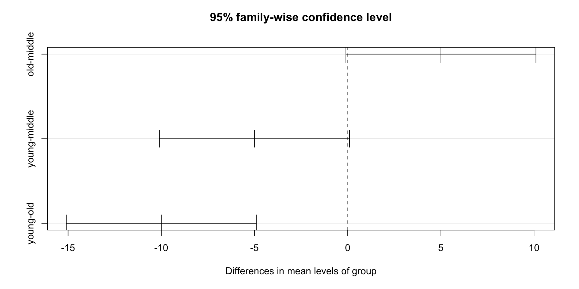
We can check how different the means of the three groups are:

Code

BP |> 
  gather(key = "group", value = "bp") |>
  aov(bp ~ group, data = _) |> 
  TukeyHSD()

  Tukey multiple comparisons of means
    95% family-wise confidence level

Fit: aov(formula = bp ~ group, data = gather(BP, key = "group", value = "bp"))

$group
             diff          lwr         upr     p adj
old-middle      5  -0.09748151 10.09748151 0.0543408
young-middle   -5 -10.09748151  0.09748151 0.0543408
young-old     -10 -15.09748151 -4.90251849 0.0010202

We can also visualize the difference:

Code

BP |> 
  gather(key = "group", value = "bp") |>
  aov(bp ~ group, data = _) |> 
  TukeyHSD() |> 
  plot()

We can see that the main difference is between the young and old groups.

4 Example

We used a very simple example to show how to calculate f-value. Now, let’s use a real data set to do the same thing. We use gapminder data set to compare the life expectancy of three different continents: Asia, Europe, and Americas.
First, let’s visualize the data:

Code

gapminder |> 
  filter(year == 2007,
         continent %in% c("Asia", "Europe", "Americas")) |> 
  ggplot(aes(x = continent, y = lifeExp)) +
  geom_boxplot()

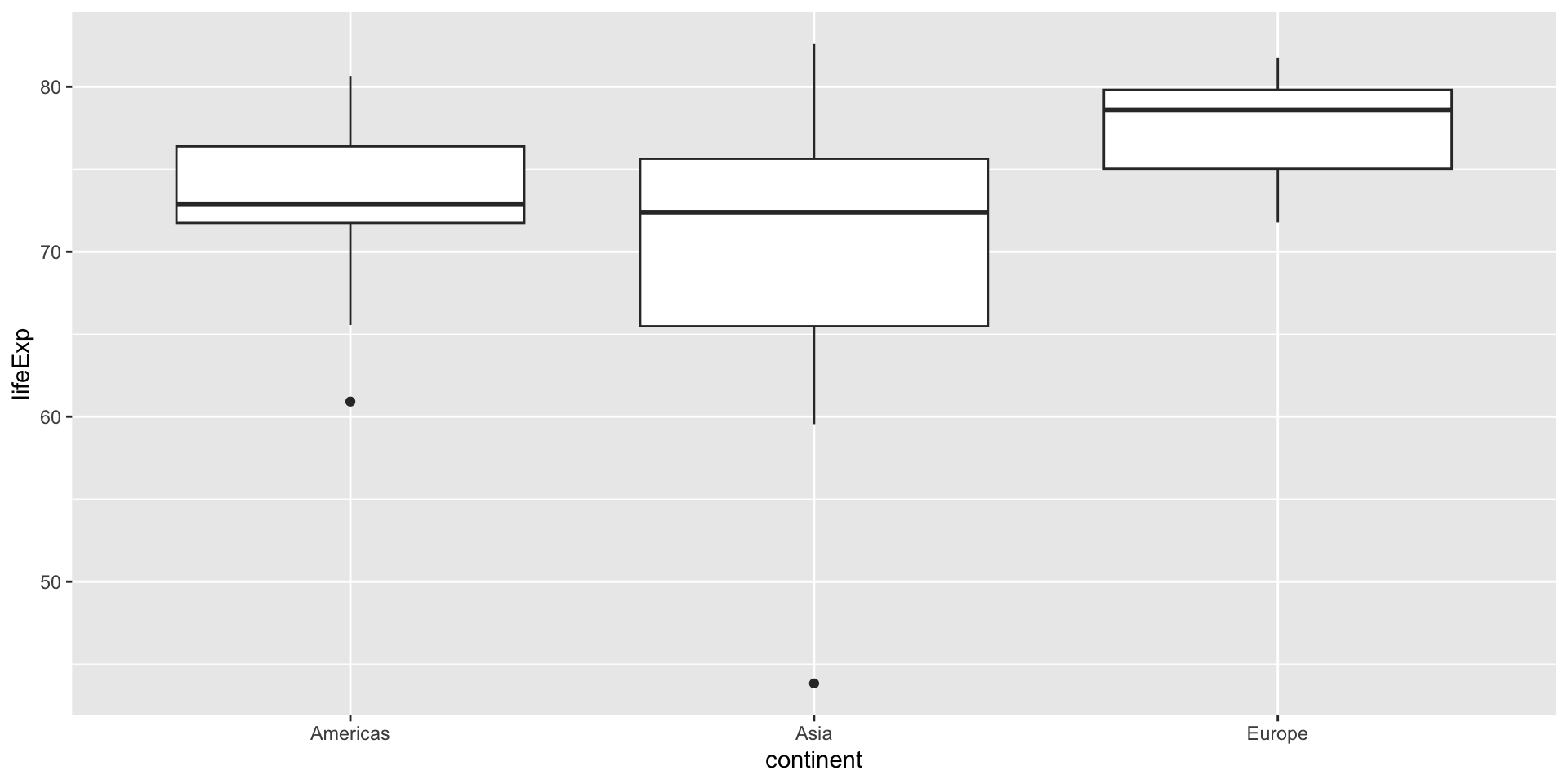
According to the boxplot, we make our hypothesis:
- H0: The mean life expectancy is the same across the three continents.
- H1: The mean life expectancy differs at least for one continent among the three.
We use R to do the test:

Code

gapminder |> 
  filter(year == 2007,
         continent %in% c("Asia", "Europe", "Americas")) |> 
  aov(lifeExp ~ continent, data = _) |> 
  summary()

            Df Sum Sq Mean Sq F value   Pr(>F)    
continent    2  755.6   377.8   11.63 3.42e-05 ***
Residuals   85 2760.3    32.5                     
---
Signif. codes:  0 '***' 0.001 '**' 0.01 '*' 0.05 '.' 0.1 ' ' 1

Based on the result, we can see that the p-value is close to 0, so we reject the null hypothesis and conclude that there is a significant difference in life expectancy among the three continents.
Which and how different?

Code

gapminder |> 
  filter(year == 2007,
         continent %in% c("Asia", "Europe", "Americas")) |> 
  aov(lifeExp ~ continent, data = _) |> 
  TukeyHSD()

  Tukey multiple comparisons of means
    95% family-wise confidence level

Fit: aov(formula = lifeExp ~ continent, data = filter(gapminder, year == 2007, continent %in% c("Asia", "Europe", "Americas")))

$continent
                     diff        lwr        upr     p adj
Asia-Americas   -2.879635 -6.4839802  0.7247099 0.1432634
Europe-Americas  4.040480  0.3592746  7.7216854 0.0279460
Europe-Asia      6.920115  3.4909215 10.3493088 0.0000189

As we can see, the main difference is between Europe and the other two continents, which is the same as we can see from the boxplot.

5 Two-Way ANOVA

In the above example, we only consider the ages which divided by three groups. If we also consider the gender, then we need to use two-way ANOVA.

Code

penguins |> 
  filter(year == 2009) |> 
  select(bill_length_mm, species, sex) |> 
  drop_na() |> 
  ggplot(aes(x = bill_length_mm, color = species)) +
  geom_boxplot() +
  facet_wrap(~ sex)

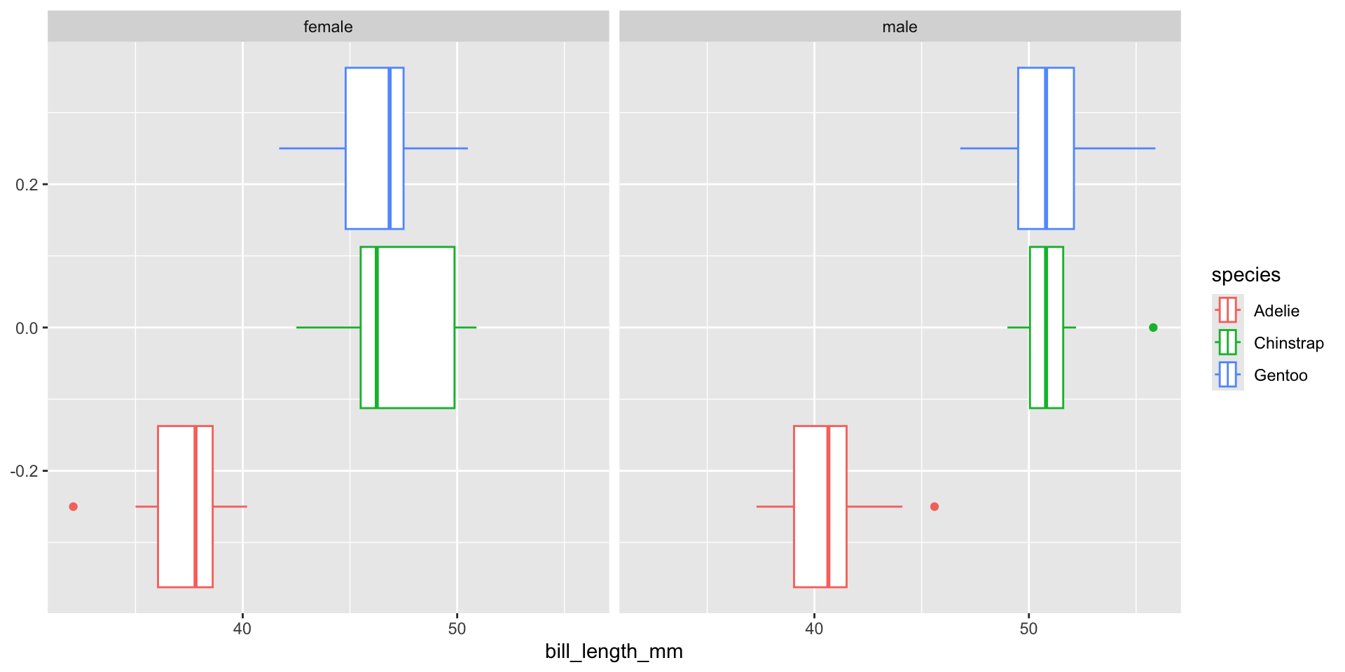
Seen from the plots, in two-way ANOVA, we not only compare among species, also compare between sexes.
Research questions
- Is there a significant difference in bill length across different species?
- Do male and female penguins exhibit variations in bill length?
- Is there a statistically significant interaction effect between species and sex concerning bill length?
Hypothese
- Research Question 1: Is there a significant difference in bill length across different species?
  - Null Hypothesis (H0): The mean bill length is the same across all species.
  - Alternative Hypothesis (H1): There is a significant difference in the mean bill length among different species.
- Research Question 2: Do male and female individuals exhibit variations in bill length?
  - Null Hypothesis (H0): There is no difference in the mean bill length between male and female individuals.
  - Alternative Hypothesis (H1): There is a significant difference in the mean bill length between male and female individuals.
- Research Question 3: Is there a statistically significant interaction effect between species and sex concerning bill length?
  - Null Hypothesis (H0): There is no interaction effect between species and sex on bill length.
  - Alternative Hypothesis (H1): There is a statistically significant interaction effect between species and sex concerning bill length.
We use R to do the test:

Code

penguins |> 
  filter(year == 2009) |> 
  drop_na(sex) |> 
  aov(bill_length_mm ~ species * sex, data = _) |> 
  summary()

             Df Sum Sq Mean Sq F value Pr(>F)    
species       2 2778.3  1389.2 299.861 <2e-16 ***
sex           1  435.4   435.4  93.979 <2e-16 ***
species:sex   2   12.8     6.4   1.382  0.255    
Residuals   111  514.2     4.6                   
---
Signif. codes:  0 '***' 0.001 '**' 0.01 '*' 0.05 '.' 0.1 ' ' 1

Based on the result, we can see that the p-value is close to 0, so we reject the null hypothesis and conclude that there is a significant difference in bill length among the three species.
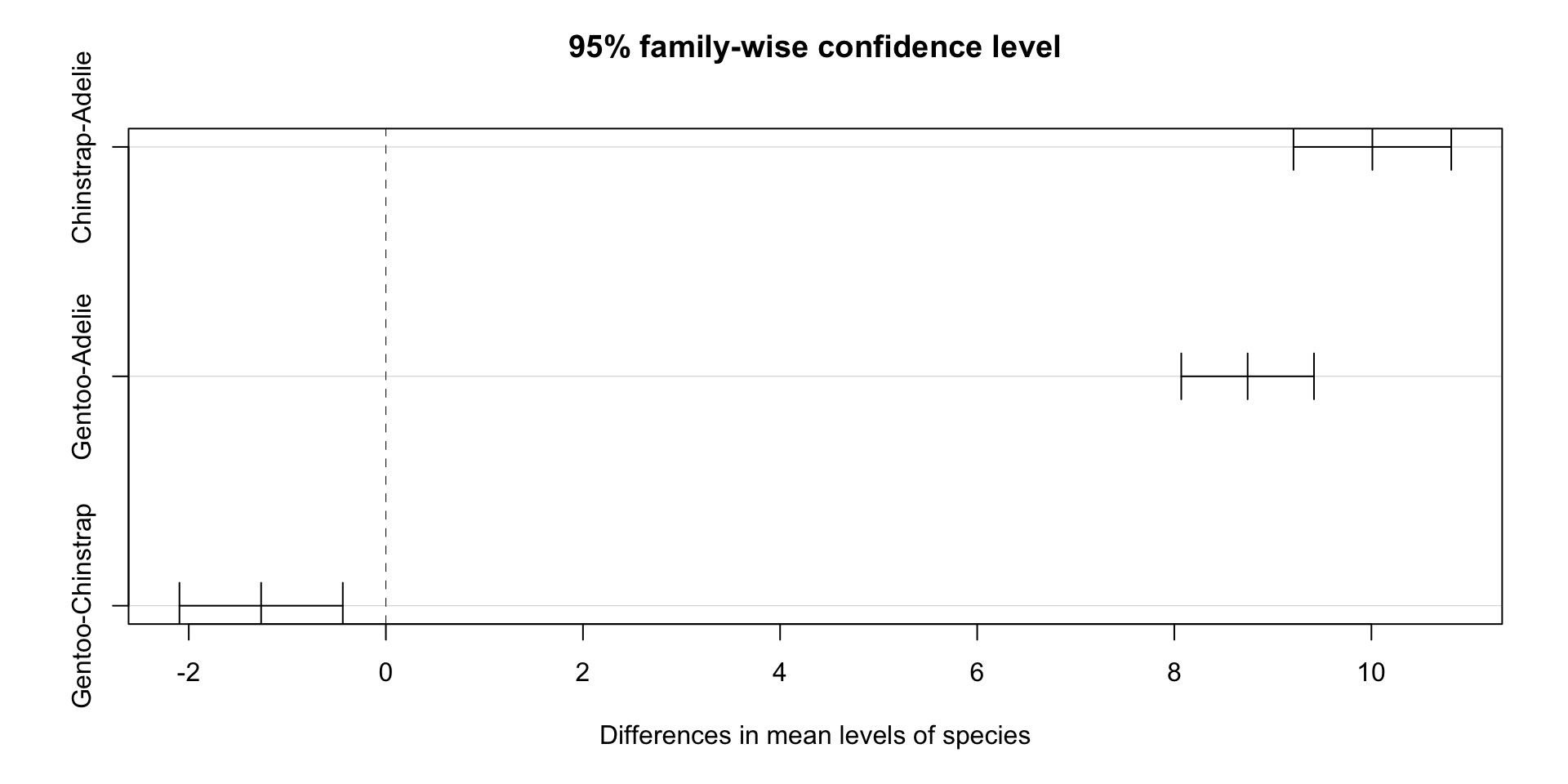
Which and how different?

Code

penguins |> 
  drop_na(sex) |> 
  aov(bill_length_mm ~ species * sex, data = _) |> 
  TukeyHSD()

  Tukey multiple comparisons of means
    95% family-wise confidence level

Fit: aov(formula = bill_length_mm ~ species * sex, data = drop_na(penguins, sex))

$species
                      diff       lwr        upr     p adj
Chinstrap-Adelie 10.009851  9.209424 10.8102782 0.0000000
Gentoo-Adelie     8.744095  8.070779  9.4174106 0.0000000
Gentoo-Chinstrap -1.265756 -2.094535 -0.4369773 0.0010847

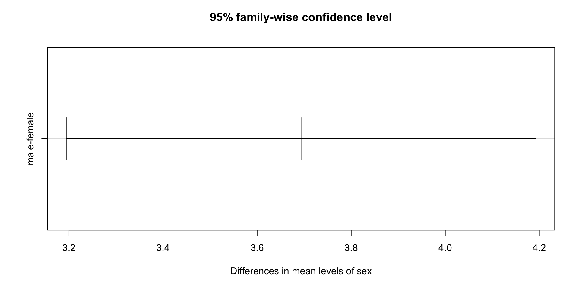
$sex
                diff      lwr      upr p adj
male-female 3.693368 3.194089 4.192646     0

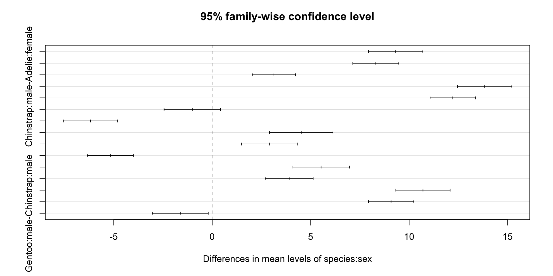
$`species:sex`
                                     diff       lwr        upr     p adj
Chinstrap:female-Adelie:female   9.315995  7.937732 10.6942588 0.0000000
Gentoo:female-Adelie:female      8.306259  7.138639  9.4738788 0.0000000
Adelie:male-Adelie:female        3.132877  2.034137  4.2316165 0.0000000
Chinstrap:male-Adelie:female    13.836583 12.458320 15.2148470 0.0000000
Gentoo:male-Adelie:female       12.216236 11.064727 13.3677453 0.0000000
Gentoo:female-Chinstrap:female  -1.009736 -2.443514  0.4240412 0.3338130
Adelie:male-Chinstrap:female    -6.183118 -7.561382 -4.8048548 0.0000000
Chinstrap:male-Chinstrap:female  4.520588  2.910622  6.1305547 0.0000000
Gentoo:male-Chinstrap:female     2.900241  1.479553  4.3209291 0.0000002
Adelie:male-Gentoo:female       -5.173382 -6.341002 -4.0057622 0.0000000
Chinstrap:male-Gentoo:female     5.530325  4.096547  6.9641020 0.0000000
Gentoo:male-Gentoo:female        3.909977  2.692570  5.1273846 0.0000000
Chinstrap:male-Adelie:male      10.703707  9.325443 12.0819703 0.0000000
Gentoo:male-Adelie:male          9.083360  7.931851 10.2348686 0.0000000
Gentoo:male-Chinstrap:male      -1.620347 -3.041035 -0.1996591 0.0149963

As we can see, except one interact is not significant, all other within and interacts are significant.
Plot

Code

penguins |> 
  drop_na(sex) |> 
  aov(bill_length_mm ~ species * sex, data = _) |> 
  TukeyHSD() |> 
  plot()

6 Repeated Measures ANOVA (Paired ANOVA)

Repeated measures ANOVA analyses the effects of one or more within-subjects (repeated measures) factors on a dependent variable. It’s used when the same subjects are measured multiple times under different conditions. It’s like a paired t-test, but for more than two conditions.

Code

gapminder |> 
  filter(year  %in% c(1952, 1982, 2007)) |> 
  mutate(year = as.factor(year)) |>
  ggplot(aes(x = year, y = lifeExp)) +
  geom_boxplot()

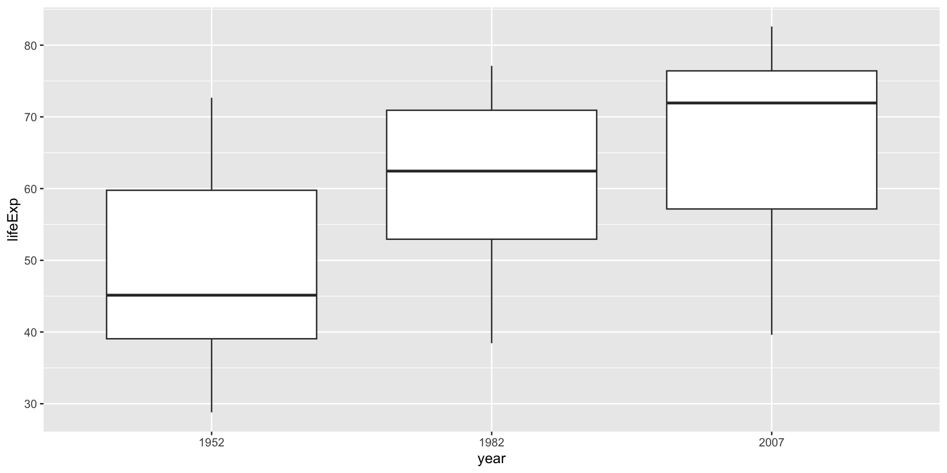
Now we use R to do the test:

Code

gapminder |> 
  filter(year  %in% c(1952, 1982, 2007)) |> 
  mutate(year = as.factor(year)) |>
  aov(lifeExp ~ year + Error(country/year), data = _) |> 
  summary()


Error: country
           Df Sum Sq Mean Sq F value Pr(>F)
Residuals 141  52225   370.4               

Error: country:year
           Df Sum Sq Mean Sq F value Pr(>F)    
year        2  24036   12018   588.4 <2e-16 ***
Residuals 282   5760      20                   
---
Signif. codes:  0 '***' 0.001 '**' 0.01 '*' 0.05 '.' 0.1 ' ' 1

Based on the result, we can see that the p-value is close to 0, so we reject the null hypothesis and conclude that there is a significant difference in life expectancy among the three years.

7 Assumptions

ANOVA has assumptions that need to be met, including the normality of data, homogeneity of variances, and independence of observations. Violation of these assumptions might affect the reliability of the ANOVA results.
- Normality: The dependent variable should be approximately normally distributed for each group of the independent variable.
- Homogeneity of variances: The variance of the dependent variable should be approximately equal for each group of the independent variable.
- Independence: The observations should be independent of each other.
We can use R to check the assumptions. If the assumptions are not met, we can use non-parametric tests, such as Kruskal-Wallis test, to do the test.

8 Recap

In this lesson, we learned:
- One-way ANOVA
- Two-way ANOVA
- Repeated measures ANOVA
In next lesson, we will learn how to do regression analysis in R.

Thank you!