R programming for beginners (GV900)

Lesson 16: Simple linear regression

Reddy Lee

Saturday, January 20, 2024

Video of Lesson 16

1 Outline

• Correlation

• Simple linear regression

• Model and interpretation

• Output of regression

library(tidyverse)
library(patchwork)
library(gapminder)
library(gtsummary)
library(gt)
library(kableExtra)
library(flextable)
library(ggpmisc)

2 Correlation

• Concept

  • Correlation is a measure of the strength of the relationship between two numeric variables.

  • Correlation is a number between -1 and 1.

  • The closer the correlation is to 1 or -1, the stronger the relationship. The closer the correlation is to 0, the weaker the relationship.

• Formula of correlation:

\[ \begin{aligned} r = {\sum\limits_{i=1}^n (x_i - \bar{x})(y_i - \bar{y}) \over \sqrt{\sum\limits_{i=1}^n (x_i - \bar{x})^2 \sum\limits_{i=1}^n (y_i - \bar{y})^2}} \end{aligned} \]

• We can see that the correlation is related to the variance and covariance of two variables.

• We have already learned the variance of a variable is defined as:

\[ \begin{aligned} \text{Var}(X) = \frac{\sum\limits_{i=1}^n (x_i - \bar{x})^2}{n-1} \end{aligned} \] - The covariance of two variables is defined as:

\[ \begin{aligned} \text{Cov}(X,Y) = \frac{\sum\limits_{i=1}^n (x_i - \bar{x})(y_i - \bar{y})}{n-1} \end{aligned} \] - The correlation is the covariance divided by the product of the standard deviations of the two variables.

\[ \begin{aligned} r = \frac{\text{Cov}(X,Y)}{\sqrt{\text{Var}(X)\text{Var}(Y)}} \end{aligned} \]

• The correlation is a standardized measure of the covariance.

• Find correlation with R

  • We can use the cor() function to find the correlation between two variables.

  • Before we use the cor() function, let’s first take a look at the scatter plot of the two variables.

(plot1 <- mtcars |>  
  ggplot(aes(x = mpg, y = wt)) +
  geom_point(color = "purple") +
  geom_smooth(method = "lm", se = FALSE))

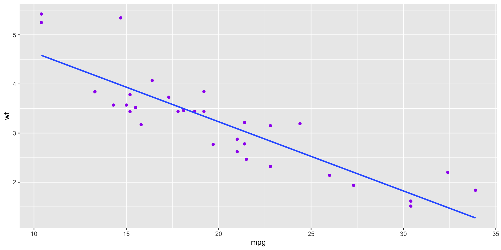
• We can conclude that there is a negative relationship between the two variables.

mtcars |> 
  select(mpg, wt) |>
  cor()

           mpg         wt
mpg  1.0000000 -0.8676594
wt  -0.8676594  1.0000000

• The correlation between mpg and wt is -0.87.

• We can see that the order of the variables does not matter.

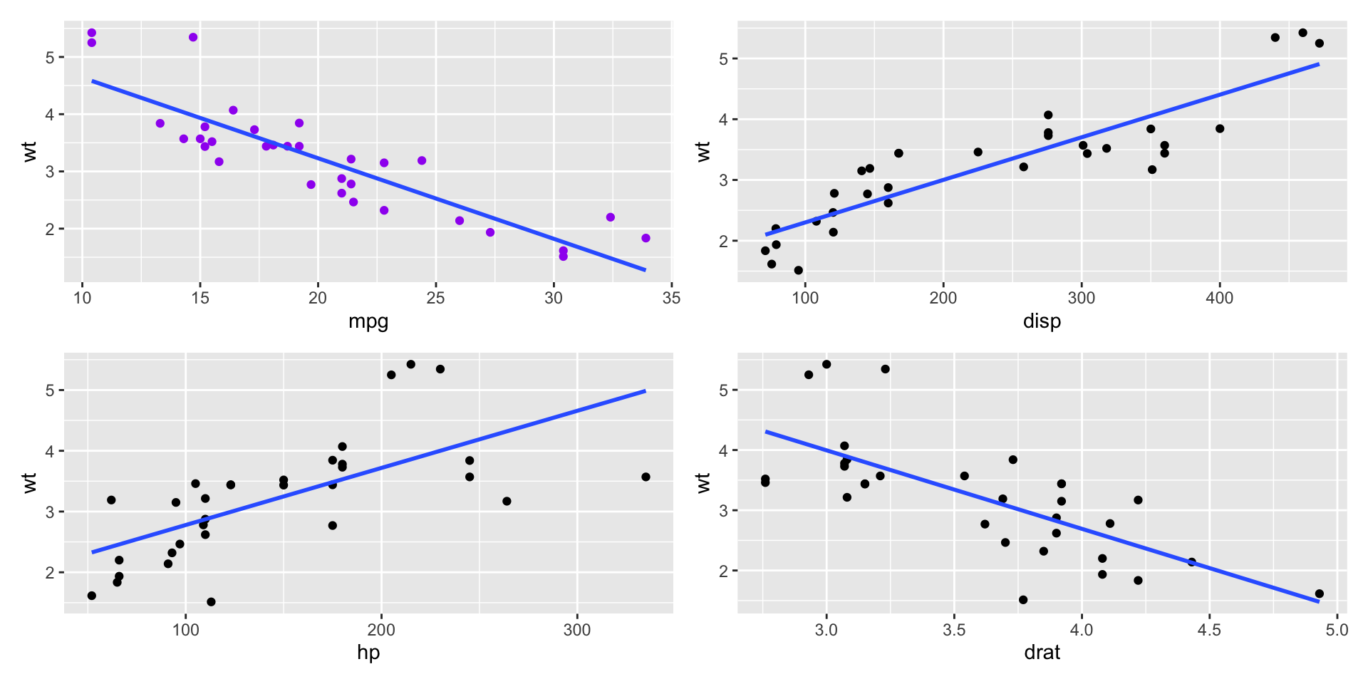
• We can find the correlation between more variables in the mtcars dataset.

  • Plots of the variables

(plot2 <- mtcars |>  
  ggplot(aes(x = disp, y = wt)) +
  geom_point() +
  geom_smooth(method = "lm", se = FALSE))

(plot3 <- mtcars |>
  ggplot(aes(x = hp, y = wt)) +
  geom_point() +
  geom_smooth(method = "lm", se = FALSE))

(plot4 <- mtcars |>
  ggplot(aes(x = drat, y = wt)) +
  geom_point() +
  geom_smooth(method = "lm", se = FALSE))

(plot5 <- mtcars |>
  ggplot(aes(x = qsec, y = wt)) +
  geom_point() +
  geom_smooth(method = "lm", se = FALSE))

• Correlation matrix

mtcars |> 
  select(wt, mpg, disp, hp, drat, qsec) |>
  cor() |> 
  round(2)

        wt   mpg  disp    hp  drat  qsec
wt    1.00 -0.87  0.89  0.66 -0.71 -0.17
mpg  -0.87  1.00 -0.85 -0.78  0.68  0.42
disp  0.89 -0.85  1.00  0.79 -0.71 -0.43
hp    0.66 -0.78  0.79  1.00 -0.45 -0.71
drat -0.71  0.68 -0.71 -0.45  1.00  0.09
qsec -0.17  0.42 -0.43 -0.71  0.09  1.00

- We can see that the correlation between `wt` and:
`mpg` is: -0.87, which is strong negative;
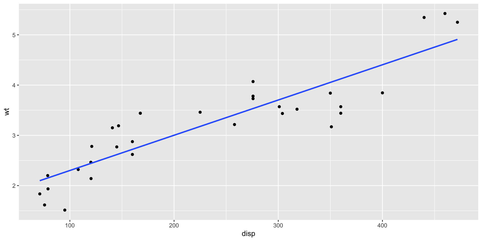
`disp` is: 0.89, which is strong positive;
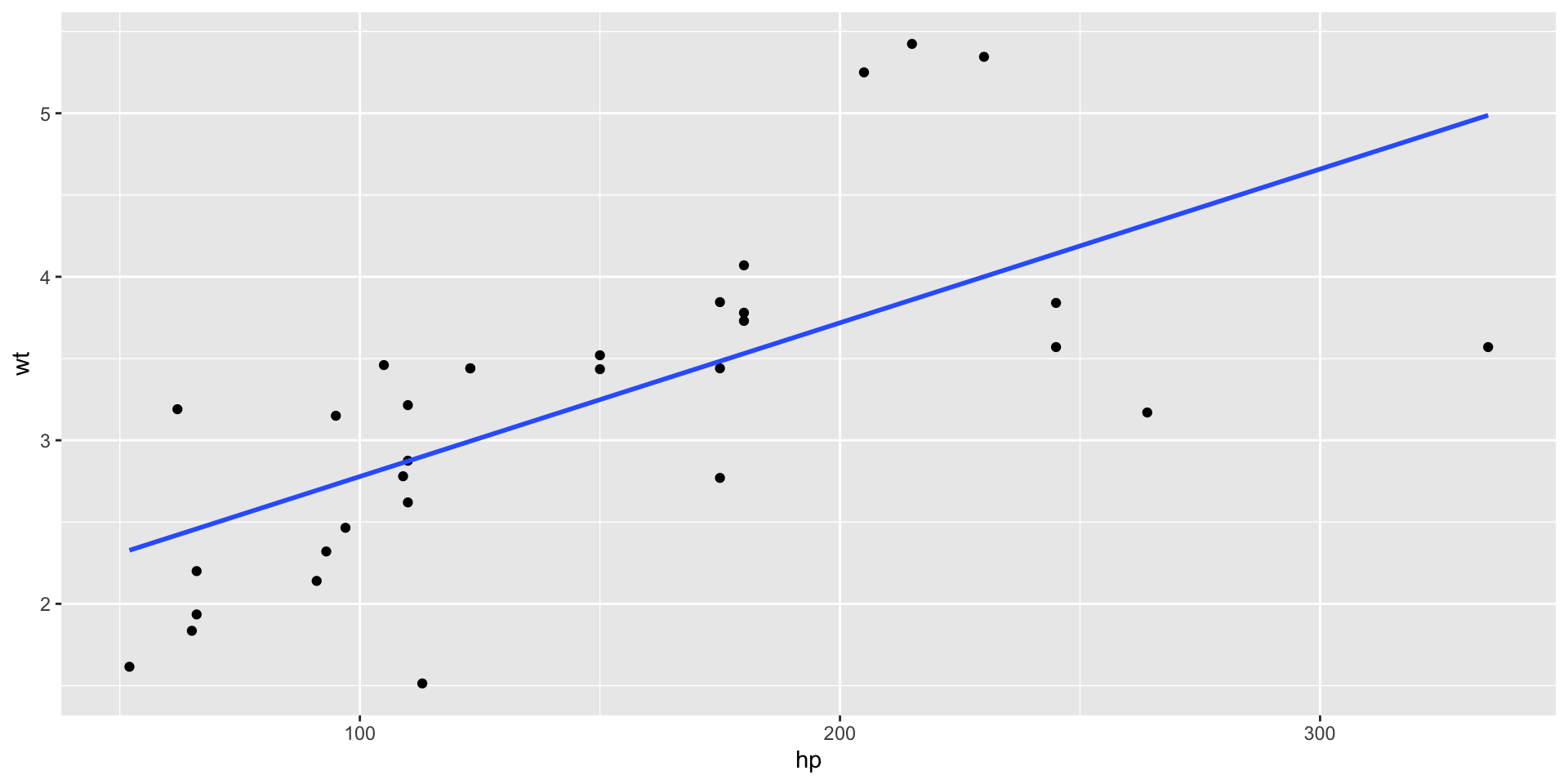
`hp` is: 0.66, which is moderate positive;
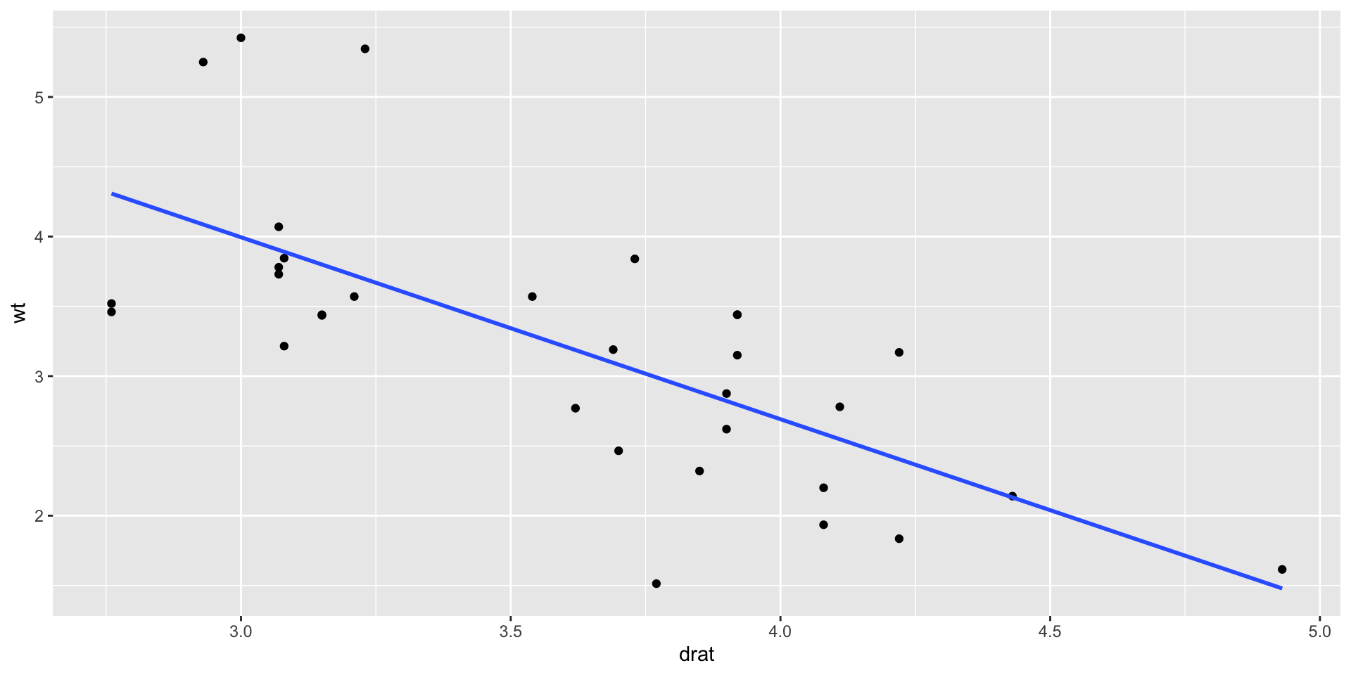
`drat` is: -0.71, which is moderate negative;
`qsec` is: -0.17, which is close to zero.

- Correlation matrix is symmetric.

- Correlation matrix plots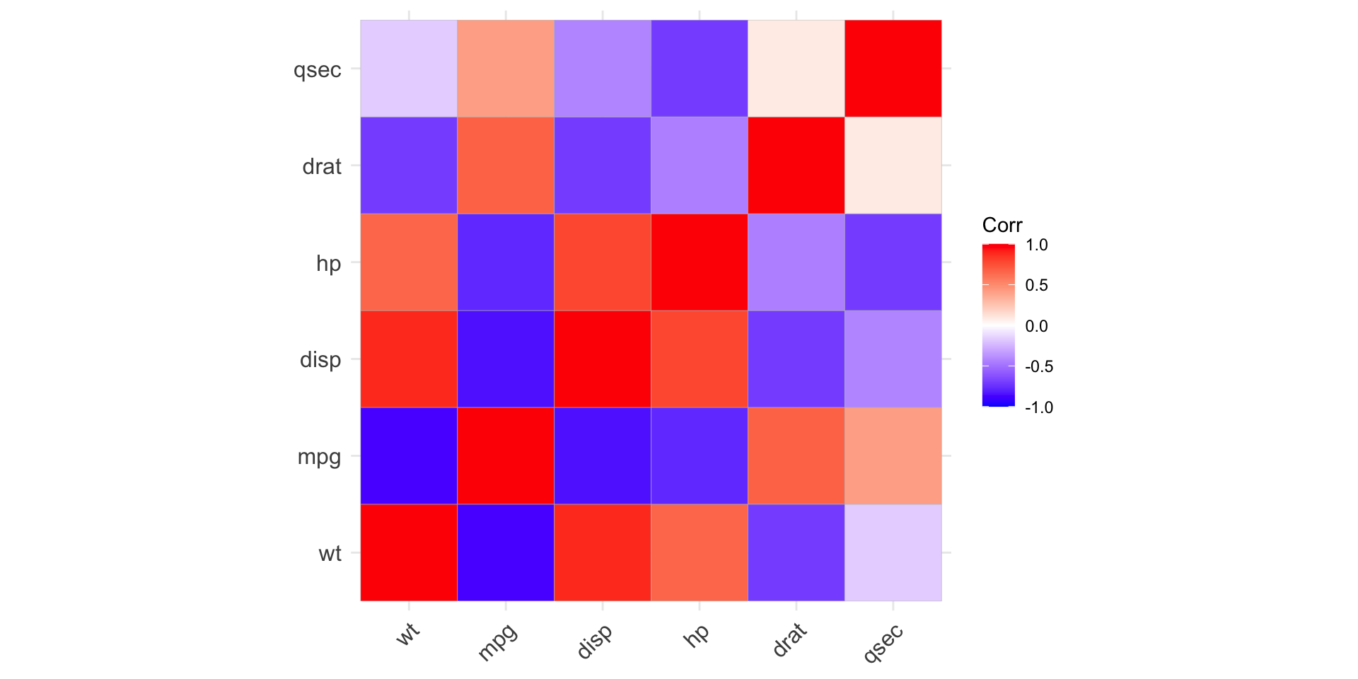

mtcars |> 
  select(wt, mpg, disp, hp, drat, qsec) |>
  cor() |> 
  ggcorrplot::ggcorrplot()

• Let’s use patchwork package to put the plots in one figure

plot1 + plot2 + plot3 + plot4

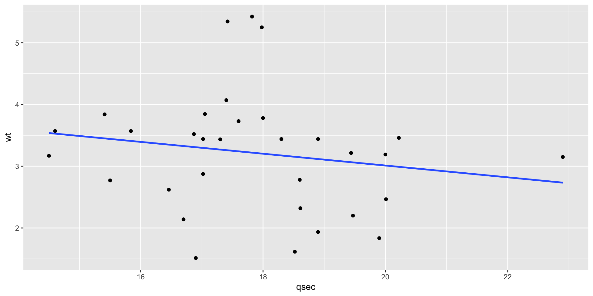
• Since the correlation between wt and qsec is -0.17, we can use cor.test() to test the correlation.

cor.test(mtcars$wt, mtcars$qsec)

    Pearson's product-moment correlation

data:  mtcars$wt and mtcars$qsec
t = -0.97191, df = 30, p-value = 0.3389
alternative hypothesis: true correlation is not equal to 0
95 percent confidence interval:
 -0.4933536  0.1852649
sample estimates:
       cor 
-0.1747159 

• The p-value is 0.34, which is greater than 0.05. We can conclude that the correlation between wt and qsec is not significant.

3 Simple linear regression

• We use gapminer dataset to illustrate the simple linear regression.

• Research question: Is there a relationship between life expectancy and GDP per capita? If so, what is the nature of the relationship? Which variable is the dependent variable and which is the independent variable?

• Hypothesis:

  • \(Ha\): There is a positive relationship between life expectancy and GDP per capita. The higher the GDP per capita, the higher the life expectancy.

• Model and interpretation

\[ \begin{aligned} \text{lifeExp} = \beta_0 + \beta_1 \text{gdpPercap} + \epsilon \end{aligned} \]

model <- gapminder |> 
  lm(lifeExp ~ gdpPercap, data = _)

summary(model)

Call:
lm(formula = lifeExp ~ gdpPercap, data = gapminder)

Residuals:
    Min      1Q  Median      3Q     Max 
-82.754  -7.758   2.176   8.225  18.426 

Coefficients:
             Estimate Std. Error t value Pr(>|t|)    
(Intercept) 5.396e+01  3.150e-01  171.29   <2e-16 ***
gdpPercap   7.649e-04  2.579e-05   29.66   <2e-16 ***
---
Signif. codes:  0 '***' 0.001 '**' 0.01 '*' 0.05 '.' 0.1 ' ' 1

Residual standard error: 10.49 on 1702 degrees of freedom
Multiple R-squared:  0.3407,    Adjusted R-squared:  0.3403 
F-statistic: 879.6 on 1 and 1702 DF,  p-value: < 2.2e-16

• We can see that the coefficient of gdpPerca is 7.649e-04, which means that for every $1000 increase in gdpPerca, the lifeExp will increase by 0.76 year. The p-value is 0.000, which is less than 0.05. We can conclude that the coefficient is significant. The adjusted R-squared is 0.34, which means that 34% of the variation in lifeExp can be explained by gdpPerca.

\[ \begin{aligned} \text{lifeExp} = 54.96 + 7.649\times 10^{-4} \text{gdpPercap} + \epsilon \end{aligned} \]

• We can use tbl_regression() from gtsummary to present the regression results in a table.

model |> 
  tbl_regression(intercept = T) |>
  as_gt() |>
  tab_options(table.width = pct(100),
              table.background.color = "#b4e1f0")

Table 1: GDP per capita and life expetancy

Characteristic	Beta	95% CI1	p-value
(Intercept)	54	53, 55	<0.001
gdpPercap	0.00	0.00, 0.00	<0.001
1 CI = Confidence Interval

4 Recap

• In this lesson, we learnt how to find the correlation between two variables and how to use simple linear regression to find how one variable might affect another variable and to what extent.

• In the following lesson, we will learn how to use multiple linear regression to find how multiple variables might affect the dependent variable and to what extent.

Thank you!