数据挖掘与R语言
第14讲:逻辑回归——多变量建模与变量筛选
2026年05月15日
上讲回顾
- 为什么用逻辑回归:二值因变量不能用线性回归,预测值会超出 \([0,1]\)
- 三步变换:\(P \to \text{Odds} = P/(1-P) \to \text{Logit} = \ln(\text{Odds})\);Logit 可以建线性模型
- Sigmoid 反推:\(P = 1/(1+e^{-\eta})\),将线性预测值还原为概率
- 系数解读:\(\hat\beta_j\) 是对数优势比变化;\(e^{\hat\beta_j}\) 是优势比(OR)
-
R 五步流程:
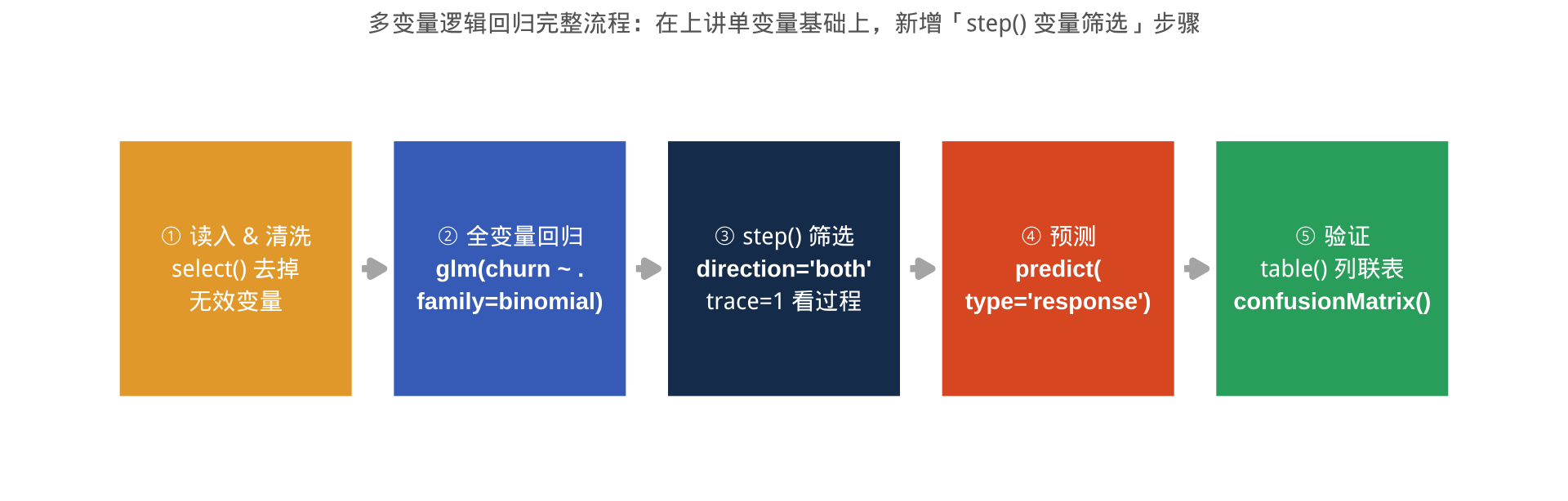
glm(family=binomial)→predict(type="response")→ifelse截断 →confusionMatrix() - 上讲只用了一个自变量(GPA)。今天加入多个变量,并学习如何自动筛选。
本讲内容
- Part 1:从单变量到多变量 ——多变量模型的结构与解读
- Part 2:电信客户流失数据 ——多变量完整演练
-
Part 3:逐步回归
step()——AIC 驱动的自动变量筛选 - Part 4:预测与评估 ——混淆矩阵与评估指标体系
- Part 5:你必须掌握什么 ——学习路线图
Part 1:从单变量到多变量
模型结构不变,变量变多了
多变量逻辑回归的模型形式
单变量时:
\[\ln\!\left(\frac{P}{1-P}\right) = \beta_0 + \beta_1 X_1\]
加入更多自变量,形式完全一样——只是右边的线性组合更长:
\[\ln\!\left(\frac{P}{1-P}\right) = \beta_0 + \beta_1 X_1 + \beta_2 X_2 + \cdots + \beta_k X_k\]
提示
偏效应(Partial Effect): 每个系数 \(\hat\beta_j\) 的含义是「控制其他变量不变,\(X_j\) 增加 1 个单位,对数优势比的变化」——与上一讲多元线性回归的偏回归系数逻辑完全相同。
注记
连续型变量和分类型变量(因子)都可以作为自变量,处理方式与线性回归完全相同:分类变量自动生成虚拟变量,第一个水平为参照组。
多变量时系数解读举例
假设模型中有两个自变量:
-
age(年龄,连续型)系数 = 0.05,OR = \(e^{0.05}\) ≈ 1.05 -
gender(性别,因子,男性为参照组)系数 = −0.40,OR = \(e^{-0.40}\) ≈ 0.67
解读:
- 控制性别不变,年龄每增加 1 岁,患病优势比增加约 5%
- 控制年龄不变,女性相比男性的患病优势比约为男性的 0.67 倍(即低约 33%)
R 代码:
Part 2:电信客户流失数据
多变量完整演练
数据介绍
数据来源: 电信客户流失数据集(churn)
▶️ 查看代码
spc_tbl_ [3,333 × 20] (S3: spec_tbl_df/tbl_df/tbl/data.frame)
 $ state                        : chr [1:3333] "KS" "OH" "NJ" "OH" ...
 $ account_length               : num [1:3333] 128 107 137 84 75 118 121 147 117 141 ...
 $ area_code                    : chr [1:3333] "area_code_415" "area_code_415" "area_code_415" "area_code_408" ...
 $ international_plan           : chr [1:3333] "no" "no" "no" "yes" ...
 $ voice_mail_plan              : chr [1:3333] "yes" "yes" "no" "no" ...
 $ number_vmail_messages        : num [1:3333] 25 26 0 0 0 0 24 0 0 37 ...
 $ total_day_minutes            : num [1:3333] 265 162 243 299 167 ...
 $ total_day_calls              : num [1:3333] 110 123 114 71 113 98 88 79 97 84 ...
 $ total_day_charge             : num [1:3333] 45.1 27.5 41.4 50.9 28.3 ...
 $ total_eve_minutes            : num [1:3333] 197.4 195.5 121.2 61.9 148.3 ...
 $ total_eve_calls              : num [1:3333] 99 103 110 88 122 101 108 94 80 111 ...
 $ total_eve_charge             : num [1:3333] 16.78 16.62 10.3 5.26 12.61 ...
 $ total_night_minutes          : num [1:3333] 245 254 163 197 187 ...
 $ total_night_calls            : num [1:3333] 91 103 104 89 121 118 118 96 90 97 ...
 $ total_night_charge           : num [1:3333] 11.01 11.45 7.32 8.86 8.41 ...
 $ total_intl_minutes           : num [1:3333] 10 13.7 12.2 6.6 10.1 6.3 7.5 7.1 8.7 11.2 ...
 $ total_intl_calls             : num [1:3333] 3 3 5 7 3 6 7 6 4 5 ...
 $ total_intl_charge            : num [1:3333] 2.7 3.7 3.29 1.78 2.73 1.7 2.03 1.92 2.35 3.02 ...
 $ number_customer_service_calls: num [1:3333] 1 1 0 2 3 0 3 0 1 0 ...
 $ churn                        : chr [1:3333] "no" "no" "no" "no" ...
 - attr(*, "spec")=
  .. cols(
  ..   state = col_character(),
  ..   account_length = col_double(),
  ..   area_code = col_character(),
  ..   international_plan = col_character(),
  ..   voice_mail_plan = col_character(),
  ..   number_vmail_messages = col_double(),
  ..   total_day_minutes = col_double(),
  ..   total_day_calls = col_double(),
  ..   total_day_charge = col_double(),
  ..   total_eve_minutes = col_double(),
  ..   total_eve_calls = col_double(),
  ..   total_eve_charge = col_double(),
  ..   total_night_minutes = col_double(),
  ..   total_night_calls = col_double(),
  ..   total_night_charge = col_double(),
  ..   total_intl_minutes = col_double(),
  ..   total_intl_calls = col_double(),
  ..   total_intl_charge = col_double(),
  ..   number_customer_service_calls = col_double(),
  ..   churn = col_character()
  .. )
 - attr(*, "problems")=<pointer: 0x7fcf00ca1bd0>
数据概况
训练集: 3333 20 测试集: 1667 20
   no   yes
0.855 0.145 注记
去掉 state(51个水平)、area_code(3个水平但无实质意义)——这两个变量要么生成过多虚拟变量,要么本身不是有效预测因子。
数据可视化:关键变量与流失的关系
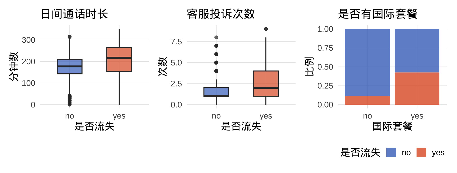
注记
流失客户日间通话时长更长、投诉更多;有国际套餐的客户流失比例明显更高——这些都是潜在的强预测变量。
步骤一:全变量逻辑回归
Call:
glm(formula = churn ~ ., family = binomial, data = train_df)

Coefficients:
                               Estimate Std. Error z value Pr(>|z|)
(Intercept)                   -8.651564   0.724314  -11.94  < 2e-16 ***
account_length                 0.000846   0.001391    0.61  0.54320
international_planyes          2.042754   0.145497   14.04  < 2e-16 ***
voice_mail_planyes            -2.025015   0.574084   -3.53  0.00042 ***
number_vmail_messages          0.035880   0.018011    1.99  0.04635 *
total_day_minutes             -0.244199   3.274222   -0.07  0.94055
total_day_calls                0.003196   0.002761    1.16  0.24705
total_day_charge               1.512708  19.260186    0.08  0.93740
total_eve_minutes              0.818695   1.635726    0.50  0.61672
total_eve_calls                0.001058   0.002783    0.38  0.70382
total_eve_charge              -9.546368  19.243727   -0.50  0.61984
total_night_minutes           -0.123829   0.876491   -0.14  0.88765
total_night_calls              0.000699   0.002842    0.25  0.80563
total_night_charge             2.833808  19.476904    0.15  0.88432
total_intl_minutes            -4.337791   5.300972   -0.82  0.41319
total_intl_calls              -0.092968   0.025060   -3.71  0.00021 ***
total_intl_charge             16.390032  19.632394    0.83  0.40380
number_customer_service_calls  0.513564   0.039268   13.08  < 2e-16 ***
---
Signif. codes:  0 '***' 0.001 '**' 0.01 '*' 0.05 '.' 0.1 ' ' 1

(Dispersion parameter for binomial family taken to be 1)

    Null deviance: 2758.3  on 3332  degrees of freedom
Residual deviance: 2158.7  on 3315  degrees of freedom
AIC: 2195

Number of Fisher Scoring iterations: 6
解读:哪些变量显著?
▶️ 查看代码
显著变量(p < 0.05):[1] "(Intercept)" "international_planyes"
[3] "voice_mail_planyes" "number_vmail_messages"
[5] "total_intl_calls" "number_customer_service_calls"注记
全变量模型包含较多不显著变量。接下来用逐步回归自动筛选,在保持预测能力的同时简化模型。
Part 3:逐步回归 step()
AIC 驱动的自动变量筛选
为什么要筛选变量?
- 过拟合风险:变量越多,模型在训练集表现越好,但泛化能力可能越差
- 多重共线性:高度相关的变量同时进入模型,系数估计不稳定
- 可解释性:变量少的模型更容易向业务方解释
提示
筛选准则:赤池信息准则(AIC)
\[\text{AIC} = -2\,\ell(\hat{\boldsymbol{\beta}}) + 2k\]
- 第一项:拟合越好(对数似然越大),AIC 越小 ✅
- 第二项:变量越多(参数数量 \(k\) 越大),AIC 越大 ❌
AIC 越小,模型越好。 它在拟合优度和模型复杂度之间取得平衡。
三种逐步策略
| 策略 | direction |
起点 | 每步操作 |
|---|---|---|---|
| 后向消除 | "backward" |
全变量模型 | 每步删除使 AIC 最小的变量 |
| 前向选择 | "forward" |
只含截距 | 每步加入能最大降低 AIC 的变量 |
| 双向逐步 | "both" |
全变量模型 | 每步可加可减,直至 AIC 不再改善 |
重要
实践中推荐 direction = "both"
双向逐步最灵活:已加入的变量可以再被删除,已删除的变量也可以再被加入。实践中通常能找到比纯后向或纯前向更优的模型。
step() 函数详解
开启 trace = 1 后,每步输出格式如下:
Step:  AIC = 856.3
churn ~ international_plan + total_day_minutes + ...

        Df  Deviance   AIC
<none>       830.3   856.3   ← 保持不变(基准)
- var_A  1   831.5   855.5   ← 删除 var_A 后 AIC 下降 → 本步删除它 ✅
- var_B  1   835.2   859.2   ← 删除 var_B 后 AIC 上升 → 保留 ❌
+ var_C  1   829.8   857.8   ← 加入 var_C 后 AIC 也上升 → 不加 ❌
提示
读懂输出的规则:
-
<none>行:当前模型 AIC 的基准值 -
-行:若该行 AIC 低于<none>→ 删除该变量能改善模型 ✅ -
+行:若该行 AIC 低于<none>→ 加入该变量能改善模型 ✅ - 每步自动执行 AIC 最小的那个操作,直到无论加减都不能降低 AIC 为止
执行逐步回归(显示过程)
逐步回归结果
Call:
glm(formula = churn ~ international_plan + voice_mail_plan +
    number_vmail_messages + total_day_charge + total_eve_minutes +
    total_night_charge + total_intl_calls + total_intl_charge +
    number_customer_service_calls, family = binomial, data = train_df)

Coefficients:
                              Estimate Std. Error z value Pr(>|z|)
(Intercept)                   -8.06716    0.51587  -15.64  < 2e-16 ***
international_planyes          2.04034    0.14524   14.05  < 2e-16 ***
voice_mail_planyes            -2.00323    0.57235   -3.50  0.00047 ***
number_vmail_messages          0.03526    0.01796    1.96  0.04965 *
total_day_charge               0.07659    0.00637   12.02  < 2e-16 ***
total_eve_minutes              0.00718    0.00114    6.29  3.2e-10 ***
total_night_charge             0.08255    0.02465    3.35  0.00081 ***
total_intl_calls              -0.09218    0.02499   -3.69  0.00023 ***
total_intl_charge              0.32614    0.07545    4.32  1.5e-05 ***
number_customer_service_calls  0.51226    0.03914   13.09  < 2e-16 ***
---
Signif. codes:  0 '***' 0.001 '**' 0.01 '*' 0.05 '.' 0.1 ' ' 1

(Dispersion parameter for binomial family taken to be 1)

    Null deviance: 2758.3  on 3332  degrees of freedom
Residual deviance: 2161.6  on 3323  degrees of freedom
AIC: 2182

Number of Fisher Scoring iterations: 6
全模型 vs 逐步回归模型
▶️ 查看代码
| 全变量模型 | 逐步回归模型 | |
|---|---|---|
| + p < 0.1, * p < 0.05, ** p < 0.01, *** p < 0.001 | ||
| (Intercept) | -8.652*** | -8.067*** |
| (-11.944) | (-15.638) | |
| account_length | 0.001 | |
| (0.608) | ||
| international_planyes | 2.043*** | 2.040*** |
| (14.040) | (14.048) | |
| voice_mail_planyes | -2.025*** | -2.003*** |
| (-3.527) | (-3.500) | |
| number_vmail_messages | 0.036* | 0.035* |
| (1.992) | (1.963) | |
| total_day_minutes | -0.244 | |
| (-0.075) | ||
| total_day_calls | 0.003 | |
| (1.158) | ||
| total_day_charge | 1.513 | 0.077*** |
| (0.079) | (12.022) | |
| total_eve_minutes | 0.819 | 0.007*** |
| (0.501) | (6.290) | |
| total_eve_calls | 0.001 | |
| (0.380) | ||
| total_eve_charge | -9.546 | |
| (-0.496) | ||
| total_night_minutes | -0.124 | |
| (-0.141) | ||
| total_night_calls | 0.001 | |
| (0.246) | ||
| total_night_charge | 2.834 | 0.083*** |
| (0.145) | (3.348) | |
| total_intl_minutes | -4.338 | |
| (-0.818) | ||
| total_intl_calls | -0.093*** | -0.092*** |
| (-3.710) | (-3.689) | |
| total_intl_charge | 16.390 | 0.326*** |
| (0.835) | (4.322) | |
| number_customer_service_calls | 0.514*** | 0.512*** |
| (13.079) | (13.087) | |
| Num.Obs. | 3333 | 3333 |
| AIC | 2194.7 | 2181.6 |
| Log.Lik. | -1079.362 | -1080.812 |
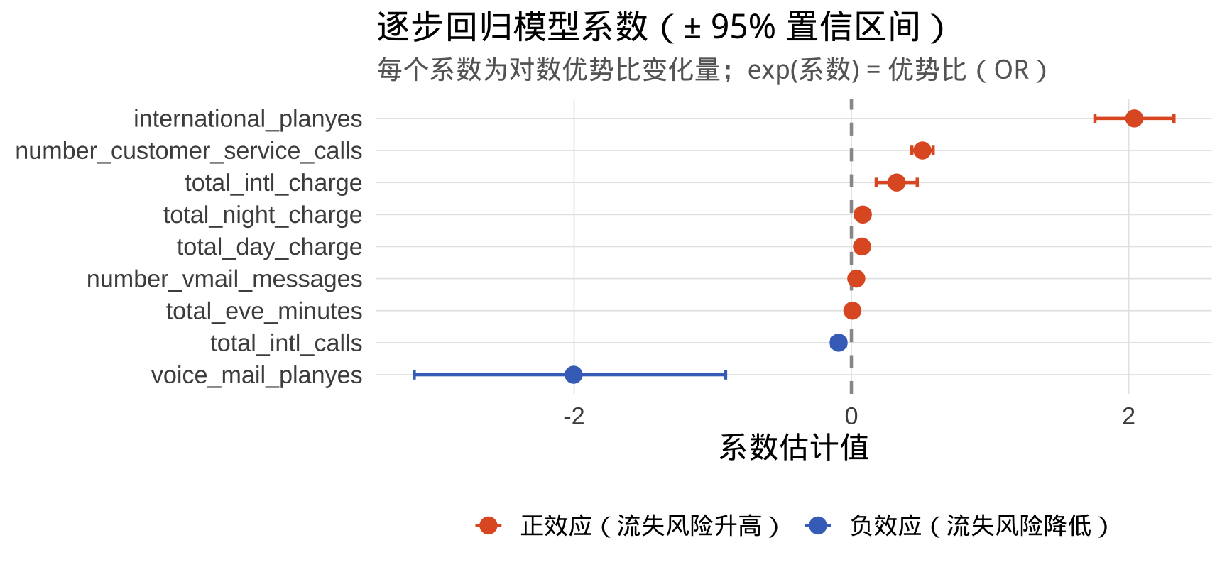
保留变量可视化
Part 4:预测与评估
混淆矩阵与评估指标体系
步骤一:在测试集上预测概率
▶️ 查看代码
   Min. 1st Qu.  Median    Mean 3rd Qu.    Max.
0.00192 0.04360 0.08523 0.14582 0.18872 0.97685 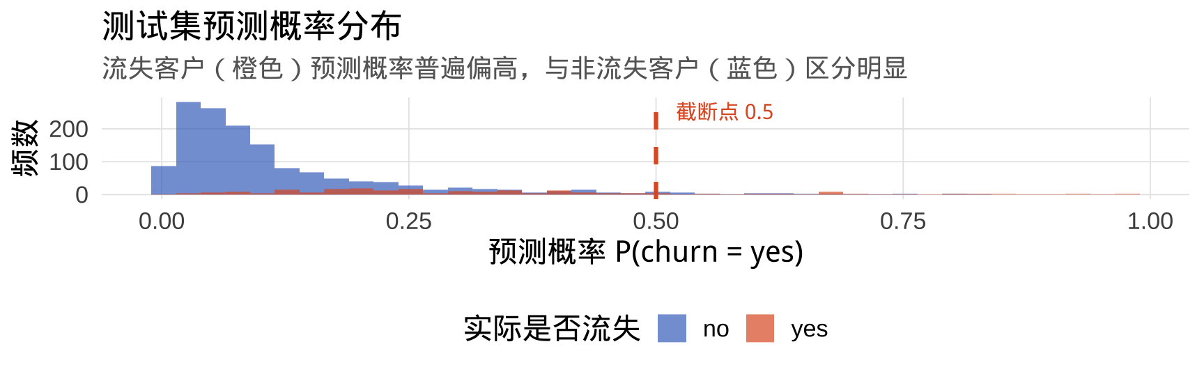
步骤二:截断处理
步骤三:混淆矩阵
      真实值
预测值   no  yes
   no  1408  182
yes 35 42| 实际:否(no) | 实际:是(yes) | |
|---|---|---|
| 预测:否(no) | TN = 1408 ✅ 正确拒识 | FN = 182 ❌ 漏报 |
| 预测:是(yes) | FP = 35 ❌ 误报 | TP = 42 ✅ 正确命中 |
四个核心指标
| 指标 | 公式 | 本模型 | 关注场景 |
|---|---|---|---|
| 准确率(Accuracy) | \((TP+TN)/N\) | 0.87 | 总体表现 |
| 灵敏度(Sensitivity) | \(TP/(TP+FN)\) | 0.188 | 漏报代价大时(如疾病筛查) |
| 特异度(Specificity) | \(TN/(TN+FP)\) | 0.976 | 误报代价大时 |
| 精确率(Precision) | \(TP/(TP+FP)\) | 0.545 | 预测为正的可信度 |
重要
灵敏度与特异度永远是一对权衡:
降低截断点 → 更多预测为"流失" → 灵敏度↑,特异度↓
升高截断点 → 更少预测为"流失" → 灵敏度↓,特异度↑
截断点选择取决于漏报(漏掉流失客户)和误报(误判不流失客户)的业务代价。
步骤四:caret::confusionMatrix() 完整评估
Confusion Matrix and Statistics

          Reference
Prediction   no  yes
       no  1408  182
       yes   35   42

               Accuracy : 0.87
                 95% CI : (0.853, 0.886)
    No Information Rate : 0.866
    P-Value [Acc > NIR] : 0.323

                  Kappa : 0.226

 Mcnemar's Test P-Value : <2e-16

            Sensitivity : 0.1875
            Specificity : 0.9757
         Pos Pred Value : 0.5455
         Neg Pred Value : 0.8855
             Prevalence : 0.1344
         Detection Rate : 0.0252
   Detection Prevalence : 0.0462
      Balanced Accuracy : 0.5816

       'Positive' Class : yes
解读评估结果
准确率(Accuracy): 0.87 Kappa 系数: 0.226 灵敏度(Sensitivity): 0.188 特异度(Specificity): 0.976 精确率(Pos Pred Value): 0.545 F1 分数: 0.279 均衡准确率(Balanced Acc.): 0.582 注记
Kappa 系数 是在排除「随机猜测」之后的一致性度量,比准确率更能反映真实能力——尤其是在类别不平衡(流失率仅 ~14%)时。
| \(\kappa\) | 一致性 |
|---|---|
| < 0.2 | 极差 |
| 0.4 ~ 0.6 | 中等 |
| > 0.8 | 高度 |
完整流程回顾
Part 5:你必须掌握什么?
学习路线图
必须掌握
重要
以下是两讲逻辑回归的完整核心,期末考试必考:
为什么逻辑回归:二值 \(Y\) 不能用线性回归;需要通过 Logit 变换建立线性模型
系数解读:对数优势比变化;\(e^{\hat\beta}\) 是 OR;OR > 1 风险升高
R 操作:
glm(y ~ ., family = binomial);summary()看显著性;exp(coef())算 OR;AIC()比较模型逐步回归:
step(model, direction = "both", trace = 1);按 AIC 自动加/删变量;读懂<none>/-/+三行的含义预测五步:
predict(type="response")→ifelse(p>0.5,...)→table()看列联表 → 分析 TP/TN/FP/FN →confusionMatrix()指标解读:准确率、灵敏度、特异度的公式与含义;Kappa 的作用;灵敏度与特异度之间的权衡
常见错误清单
警告
请对照检查:
| 错误 | 正确做法 |
|---|---|
| 把系数说成「概率变化 \(\hat\beta\)」 | 系数是对数优势比变化,概率变化需通过 Sigmoid 计算,不是常数 |
忘记 family = binomial
|
不写等于线性回归,二值 \(Y\) 完全错误 |
predict() 不写 type = "response"
|
默认输出 Logit,不是概率;要概率必须加 type = "response"
|
step() 只做后向或只做前向 |
推荐 direction = "both",结果更稳健 |
| 只看准确率就得出结论 | 类别不平衡时准确率会虚高;需同时看 Kappa 和灵敏度 |
confusionMatrix() 不指定 positive
|
正类会按字母顺序确定,可能解读颠倒 |
本讲小结
多变量逻辑回归:模型形式与单变量完全相同,只是右边线性组合更长;每个系数是偏效应
逐步回归:
step(model, direction = "both", trace = 1)按 AIC 自动筛选;读懂每步的<none>/-/+行;最终得到更简洁且 AIC 更小的模型评估体系:混淆矩阵 → 准确率 / 灵敏度 / 特异度 / Kappa;
confusionMatrix()一键计算;截断点的选择是业务决策,不是统计问题两讲合并记忆:理论(上讲)+ 单变量练习(admissions)→ 多变量建模(下讲)→
step()筛选 → 心脏病作业
课后作业
作业说明
项目介绍: 现有一组心脏病研究数据集 heart_learning(训练集)和 heart_test(测试集),包含年龄、性别、疼痛等级等 15 个变量,最后一个变量为是否心脏病的二值变量 target。以 R 语言为分析工具,以 target 为因变量,构建逻辑回归模型,并在测试集上评估准确性。
步骤 1:读入数据与基本结构
▶️ 查看代码
'data.frame':   206 obs. of  14 variables:
 $ age    : int  63 37 41 56 57 57 56 52 57 54 ...
 $ sex    : int  1 1 0 1 0 1 0 1 1 1 ...
 $ pain   : int  1 3 2 2 4 4 2 3 3 4 ...
 $ bpress : int  145 130 130 120 120 140 140 172 150 140 ...
 $ chol   : int  233 250 204 236 354 192 294 199 168 239 ...
 $ bsugar : int  1 0 0 0 0 0 0 1 0 0 ...
 $ ekg    : int  2 0 2 0 0 0 2 0 0 0 ...
 $ thalach: int  150 187 172 178 163 148 153 162 174 160 ...
 $ exang  : int  0 0 0 0 1 0 0 0 0 0 ...
 $ oldpeak: num  2.3 3.5 1.4 0.8 0.6 0.4 1.3 0.5 1.6 1.2 ...
 $ slope  : int  3 3 1 1 1 2 2 1 1 1 ...
 $ ca     : int  0 0 0 0 0 0 0 0 0 0 ...
 $ thal   : int  6 3 3 3 3 6 3 7 3 3 ...
$ target : int 0 0 0 0 0 0 0 0 0 0 ... age sex pain bpress chol
Min. :29.0 Min. :0.00 Min. :1.00 Min. : 94 Min. :126
1st Qu.:48.0 1st Qu.:0.00 1st Qu.:2.25 1st Qu.:120 1st Qu.:211
Median :55.0 Median :1.00 Median :3.00 Median :130 Median :240
Mean :54.4 Mean :0.68 Mean :3.15 Mean :132 Mean :246
3rd Qu.:61.8 3rd Qu.:1.00 3rd Qu.:4.00 3rd Qu.:140 3rd Qu.:278
Max. :77.0 Max. :1.00 Max. :4.00 Max. :192 Max. :417
bsugar ekg thalach exang oldpeak
Min. :0.000 Min. :0.00 Min. : 71 Min. :0.000 Min. :0.00
1st Qu.:0.000 1st Qu.:0.00 1st Qu.:136 1st Qu.:0.000 1st Qu.:0.00
Median :0.000 Median :2.00 Median :152 Median :0.000 Median :0.80
Mean :0.141 Mean :1.05 Mean :150 Mean :0.335 Mean :1.07
3rd Qu.:0.000 3rd Qu.:2.00 3rd Qu.:168 3rd Qu.:1.000 3rd Qu.:1.60
Max. :1.000 Max. :2.00 Max. :202 Max. :1.000 Max. :6.20
slope ca thal target
Min. :1.00 Min. :0.000 Min. :3.0 Min. :0.000
1st Qu.:1.00 1st Qu.:0.000 1st Qu.:3.0 1st Qu.:0.000
Median :2.00 Median :0.000 Median :3.0 Median :0.000
Mean :1.57 Mean :0.665 Mean :4.7 Mean :0.456
3rd Qu.:2.00 3rd Qu.:1.000 3rd Qu.:7.0 3rd Qu.:1.000
Max. :3.00 Max. :3.000 Max. :7.0 Max. :1.000
  0   1
112  94
    0     1
0.544 0.456
要求: 简要说明训练集有多少行、多少列;因变量 target 的 0 和 1 各占多少比例。
步骤 2:全变量 Logit 回归
▶️ 查看代码
Call:
glm(formula = target ~ ., family = binomial(link = "logit"),
    data = heart_learning)

Coefficients:
            Estimate Std. Error z value Pr(>|z|)
(Intercept) -7.51997    3.76964   -1.99   0.0461 *
age         -0.02416    0.03075   -0.79   0.4321
sex          1.48854    0.64491    2.31   0.0210 *
pain         0.66449    0.25046    2.65   0.0080 **
bpress       0.04025    0.01470    2.74   0.0062 **
chol         0.00929    0.00533    1.74   0.0815 .
bsugar      -1.03403    0.75565   -1.37   0.1712
ekg          0.42031    0.24952    1.68   0.0921 .
thalach     -0.03853    0.01405   -2.74   0.0061 **
exang        0.91653    0.51666    1.77   0.0761 .
oldpeak      0.54409    0.29775    1.83   0.0677 .
slope       -0.05308    0.47801   -0.11   0.9116
ca           0.88911    0.31288    2.84   0.0045 **
thal         0.43797    0.13630    3.21   0.0013 **
---
Signif. codes:  0 '***' 0.001 '**' 0.01 '*' 0.05 '.' 0.1 ' ' 1

(Dispersion parameter for binomial family taken to be 1)

    Null deviance: 284.00  on 205  degrees of freedom
Residual deviance: 127.01  on 192  degrees of freedom
AIC: 155

Number of Fisher Scoring iterations: 6
要求: 列举哪些变量的系数显著(\(p < 0.05\))、哪些不显著;指出全模型的 AIC 是多少。
步骤 3:逐步回归变量筛选
Start:  AIC=155
target ~ age + sex + pain + bpress + chol + bsugar + ekg + thalach +
    exang + oldpeak + slope + ca + thal

          Df Deviance AIC
- slope    1      127 153
- age      1      128 154
- bsugar   1      129 155
<none>            127 155
- ekg      1      130 156
- chol     1      130 156
- exang    1      130 156
- oldpeak  1      131 157
- sex      1      133 159
- pain     1      135 161
- bpress   1      135 161
- thalach  1      135 161
- ca       1      136 162
- thal     1      138 164

Step:  AIC=153
target ~ age + sex + pain + bpress + chol + bsugar + ekg + thalach +
    exang + oldpeak + ca + thal

          Df Deviance AIC
- age      1      128 152
<none>            127 153
- bsugar   1      129 153
- ekg      1      130 154
- exang    1      130 154
- chol     1      130 154
+ slope    1      127 155
- oldpeak  1      132 156
- sex      1      133 157
- pain     1      135 159
- bpress   1      135 159
- thalach  1      136 160
- ca       1      137 161
- thal     1      138 162

Step:  AIC=152
target ~ sex + pain + bpress + chol + bsugar + ekg + thalach +
    exang + oldpeak + ca + thal

          Df Deviance AIC
<none>            128 152
- bsugar   1      130 152
- ekg      1      130 152
- chol     1      130 152
- exang    1      131 153
+ age      1      127 153
+ slope    1      128 154
- oldpeak  1      133 155
- sex      1      134 156
- bpress   1      135 157
- pain     1      136 158
- thalach  1      136 158
- ca       1      137 159
- thal     1      139 161
Call:
glm(formula = target ~ sex + pain + bpress + chol + bsugar +
    ekg + thalach + exang + oldpeak + ca + thal, family = binomial(link = "logit"),
    data = heart_learning)

Coefficients:
            Estimate Std. Error z value Pr(>|z|)
(Intercept) -9.20150    3.05119   -3.02   0.0026 **
sex          1.53717    0.63515    2.42   0.0155 *
pain         0.67914    0.24758    2.74   0.0061 **
bpress       0.03714    0.01408    2.64   0.0083 **
chol         0.00861    0.00514    1.67   0.0940 .
bsugar      -1.06340    0.73708   -1.44   0.1491
ekg          0.40455    0.24376    1.66   0.0970 .
thalach     -0.03319    0.01210   -2.74   0.0061 **
exang        0.93516    0.51520    1.82   0.0695 .
oldpeak      0.56246    0.24938    2.26   0.0241 *
ca           0.85336    0.29984    2.85   0.0044 **
thal         0.43429    0.13534    3.21   0.0013 **
---
Signif. codes:  0 '***' 0.001 '**' 0.01 '*' 0.05 '.' 0.1 ' ' 1

(Dispersion parameter for binomial family taken to be 1)

    Null deviance: 284.00  on 205  degrees of freedom
Residual deviance: 127.65  on 194  degrees of freedom
AIC: 151.7

Number of Fisher Scoring iterations: 6
要求: 说明逐步回归最终保留了多少变量;最终模型 AIC 是多少;与全变量模型相比 AIC 如何变化。
步骤 4:预测与混淆矩阵
▶️ 查看代码
      预测值
真实值  0  1
     0 41  7
     1 10 33
要求: 指出 TP、TN、FP、FN 各是多少;计算准确率;分析模型在漏诊(FN)和误诊(FP)上的表现。
步骤 5:caret 完整评估
▶️ 查看代码
Confusion Matrix and Statistics


     0  1
  0 41 10
  1  7 33

               Accuracy : 0.813
                 95% CI : (0.718, 0.887)
    No Information Rate : 0.527
    P-Value [Acc > NIR] : 1.24e-08

                  Kappa : 0.624

 Mcnemar's Test P-Value : 0.628

            Sensitivity : 0.767
            Specificity : 0.854
         Pos Pred Value : 0.825
         Neg Pred Value : 0.804
             Prevalence : 0.473
         Detection Rate : 0.363
   Detection Prevalence : 0.440
      Balanced Accuracy : 0.811

       'Positive' Class : 1
要求: 报告并解读以下指标:
- 准确率(Accuracy)
- 灵敏度(Sensitivity)——正确识别心脏病患者的比例
- 特异度(Specificity)——正确识别健康人的比例
- Kappa 系数
谢谢!
第14讲:多变量逻辑回归
「所有模型都是错的,但有些是有用的。」
—— 乔治·博克斯(George Box)
数据挖掘与R语言 | 第14讲:多变量逻辑回归