数据挖掘与R语言

第22讲：关联规则（二）——参数调优、可视化与购物篮分析实战

朱 奇

2026年06月12日

上讲回顾

• 关联规则：形如 \(A \Rightarrow B\)，描述项目的共现模式（相关性，非因果）
• 三大度量指标：
  • 支持度 \(P(A \cap B)\)——规则出现的频率，筛选频繁项集
  • 置信度 \(P(B \mid A)\)——规则的预测可靠性
  • 提升度 \(\dfrac{P(A \cap B)}{P(A) \cdot P(B)}\)——排除畅销品干扰，> 1 才有价值
• Apriori 算法：利用反单调性逐层剪枝，\(L_k \to C_{k+1} \to L_{k+1}\)，大幅削减候选集数量
• R 实现：arules::apriori() 挖掘规则，arulesViz 可视化
• 今天：学习参数精细调优、规则精准筛选，以及购物篮分析综合实战

本讲内容

• 第 1 部分：知识点回顾与重难点导入（10 分钟）
• 第 2 部分：R 语言实战——Apriori 参数调优与规则筛选（20 分钟）
• 第 3 部分：图形化展示——散点图与网络图（15 分钟）
• 第 4 部分：综合练习——零售超市购物篮分析（35 分钟）
• 第 5 部分：课程总结（10 分钟）

第 1 部分：回顾与衔接

重难点导入——提升度的正确使用

互动提问：置信度高就够了吗？

重要

课堂提问

一条规则的置信度是 90%，但提升度只有 0.8，这条规则有价值吗？

答案：没有价值。

• 置信度 90% 看似可靠，但提升度 0.8 < 1，说明 \(A\) 实际上抑制了 \(B\) 的出现
• 即：知道顾客买了 \(A\) 之后，\(B\) 的购买概率反而低于它本来的基础概率
• 这条规则不但没用，还会误导决策（例如错误地将 A 和 B 相邻陈列）

提示

今天的核心目标

学习如何通过 R 语言代码，自动过滤垃圾规则，精准定位真正有价值的关联规律。

三大指标速查表

第 2 部分：R 语言实战

Apriori 参数调优与规则精准筛选

基础建模：apriori() 参数一览

最基本的调用形式：

library(arules)

rules <- apriori(
  data,
  parameter = list(
    support    = 0.01,   # 最小支持度
    confidence = 0.5,    # 最小置信度
    minlen     = 2       # 规则最少含几个项（默认1，建议设为2排除空规则）
  )
)

注记

参数调优的出发点

参数	调低	调高
support	规则更多，但噪声增加	规则减少，只保留普遍规律
confidence	可靠性门槛降低	只保留高可靠性规则
minlen	包含单项规则（意义不大）	强制要求前后项都存在

精确筛选：subset() 定向分析

核心函数：用条件表达式从规则集中提取子集

# 筛选后项包含"Audit_Risk"的所有规则（"什么会导致审计风险？"）
risks_rules <- subset(rules, items %in% "Audit_Risk")

# 只看前项（lhs）包含某项的规则
lhs_rules <- subset(rules, lhs %in% "商品A")

# 只看后项（rhs）包含某项的规则
rhs_rules <- subset(rules, rhs %in% "商品B")

# 组合条件：lift 大于 2 且 confidence 大于 0.7
strong_rules <- subset(rules, lift > 2 & confidence > 0.7)

提示

items %in% 匹配前项或后项中含有指定商品的规则（不区分左右）；

lhs %in% 只匹配前项；rhs %in% 只匹配后项。

排序：按提升度找最有价值的规则

挖掘规则后，第一步永远是按提升度降序排列：

# 按提升度从高到低排序
rules_sorted <- sort(rules, by = "lift", decreasing = TRUE)

# 查看前 10 条最有价值的规则
inspect(rules_sorted[1:10])

典型输出示例（Groceries 数据集）：

   lhs                         rhs                support confidence    lift
1  {citrus fruit,              => {root vegetables}  0.010      0.586   5.38
    root vegetables}
2  {tropical fruit,            => {other vegetables} 0.012      0.712   3.68
    yogurt}
...

重要

黄金法则：先排序提升度，再看置信度，最后看支持度。 高提升度 + 高置信度 + 合理支持度 = 真正值得关注的规则。

完整工作流演示

library(arules)
data("Groceries")

# Step 1：挖掘规则
rules <- apriori(
  Groceries,
  parameter = list(support = 0.005, confidence = 0.4, minlen = 2)
)

# Step 2：按提升度排序，查看最优规则
rules_by_lift <- sort(rules, by = "lift")
inspect(head(rules_by_lift, 10))

# Step 3：定向筛选——找所有导致"whole milk"被购买的规则
milk_rules <- subset(rules, rhs %in% "whole milk" & lift > 1.5)
inspect(sort(milk_rules, by = "lift"))

注记

inspect() 是 arules 包的专用函数，以友好格式打印规则列表，等同于对规则集的 print()。

课堂互动：参数调整的权衡

重要

思考题

在 Groceries 数据集上，如果把 support 从 0.005 调高到 0.05， 结果会发生什么变化？

1. 规则数量会增加还是减少？
2. 平均提升度会变高还是变低？为什么？

• 规则数量减少：更高的支持度门槛只保留普遍出现的商品组合，长尾关联被过滤
• 平均提升度可能降低：高支持度的项集往往是本就畅销的商品，相互之间的提升度趋近于 1
• 结论：min_sup 设置需要结合业务目标——探索阶段宜宽松，汇报阶段宜严格

第 3 部分：关联规则可视化

arulesViz——散点图与网络图

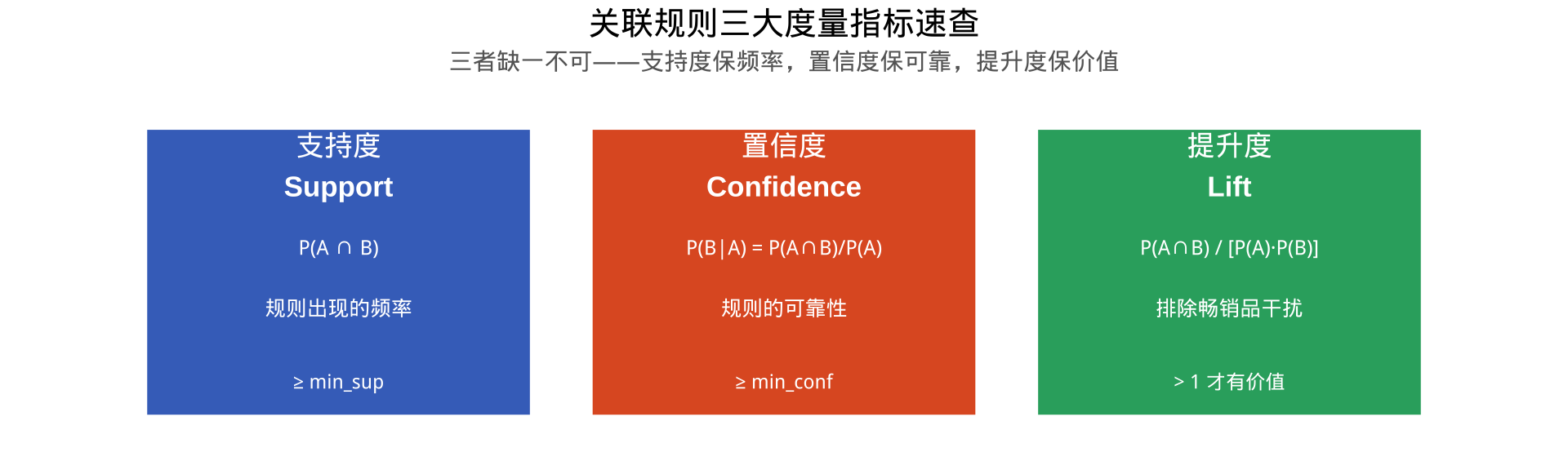
散点图：三指标全景鸟瞰

library(arulesViz)

# 散点图：x = 支持度，y = 置信度，颜色深浅 = 提升度
plot(
  rules,
  measure = c("support", "confidence"),
  shading = "lift",
  main    = "关联规则散点图（颜色越深 = 提升度越高）"
)

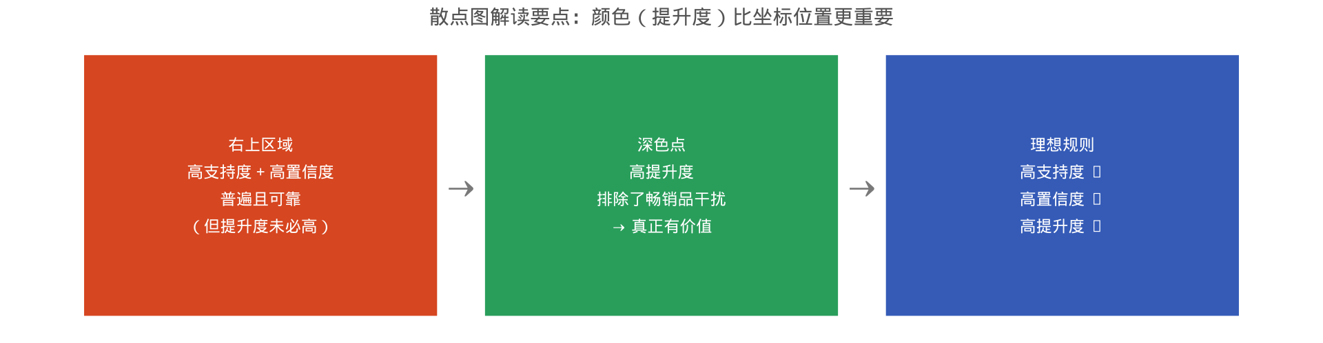
如何阅读散点图？

网络图：直观展示商品关联结构

# 取提升度最高的 30 条规则绘制网络图
top30 <- sort(rules, by = "lift")[1:30]

plot(
  top30,
  method = "graph",
  engine = "htmlwidget"   # 交互式；改为 "igraph" 输出静态图
)

网络图的阅读方式：

• 节点（圆球）：代表商品，节点越大说明该商品的支持度越高（越畅销）
• 边（箭头）：代表一条关联规则，箭头从前项指向后项
• 颜色深浅：颜色越深，提升度越高，规则越有价值
• 聚集性：紧密相连的商品群体往往对应同一消费场景（早餐、烘焙、健康饮食等）

网络图的业务解读

提示

实际案例：超市购物篮网络图的典型发现

注记

财务审计场景的延伸

在财务审计中，网络图可以直观展示哪些违规行为是"成群结队"出现的——例如"虚增收入"节点与"应收账款异常"节点之间若有深色粗边，说明两者高度关联，需要联合排查。

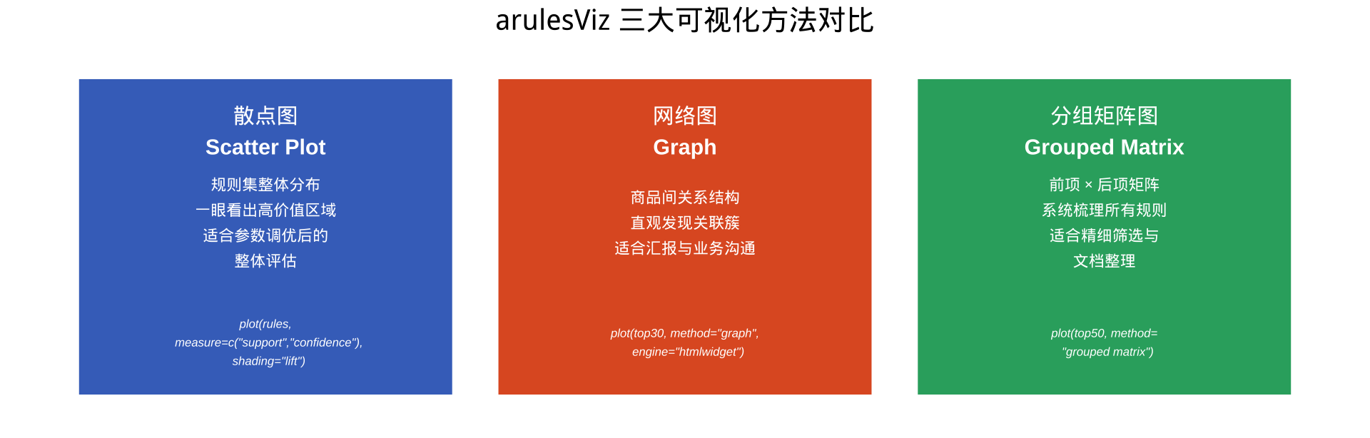
可视化方法对比

第 4 部分：综合练习

实训 ——零售超市购物篮分析与交叉销售建议

实训数据介绍

数据文件：data.txt（4 笔事务，5 种商品）

实训数据集（N = 4 笔事务，商品代码：X、Y、Z、M、N）

事务ID	购买商品	商品数
T1	X, Z, M	3
T2	Y, Z, N	3
T3	X, Y, Z, N	4
T4	Y, N	2

数据格式说明：

X,Z,M
Y,Z,N
X,Y,Z,N
Y,N

• 每行为一笔事务，商品代码用英文逗号分隔
• 读入方式：read.transactions("data.txt", format = "basket", sep = ",")

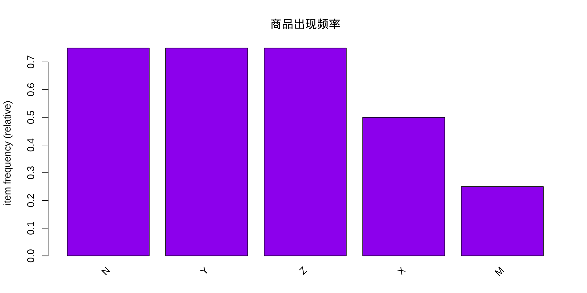
练习 1：读入数据与摘要分析

目标：了解数据集的基本结构与商品分布

library(arules)
library(arulesViz)

# 读入数据
trans <- read.transactions(
  "data.txt",
  format = "basket",   # 每行为一笔购物篮
  sep    = ","         # 商品用逗号分隔
)

# 查看基本摘要
summary(trans)

transactions as itemMatrix in sparse format with
 4 rows (elements/itemsets/transactions) and
 5 columns (items) and a density of 0.6 

most frequent items:
      N       Y       Z       X       M (Other) 
      3       3       3       2       1       0 

element (itemset/transaction) length distribution:
sizes
2 3 4 
1 2 1 

   Min. 1st Qu.  Median    Mean 3rd Qu.    Max. 
   2.00    2.75    3.00    3.00    3.25    4.00 

includes extended item information - examples:
  labels
1      M
2      N
3      X

# 查看每种商品的支持度（出现频率）
itemFrequency(trans)

   M    N    X    Y    Z 
0.25 0.75 0.50 0.75 0.75 

# 绘制商品频率条形图
itemFrequencyPlot(trans, 
                  topN   = 5, 
                  support = 0.1, 
                  main = "商品出现频率",
                  col = "purple")

提示

summary() 会告诉你什么？

事务总数、商品总数、最短/最长事务长度，以及最常出现的商品排名。

练习 1：预期输出解读

各商品支持度一览（N = 4）

商品	出现次数	支持度	备注
X	2	2/4 = 0.50	T1、T3
Y	3	3/4 = 0.75	T2、T3、T4
Z	3	3/4 = 0.75	T1、T2、T3
M	1	1/4 = 0.25	仅 T1
N	3	3/4 = 0.75	T2、T3、T4

注记

观察：Y、Z、N 的支持度均为 75%，是本数据集的高频商品； M 支持度仅 25%，在高 min_sup 阈值下将被过滤。

练习 2：挖掘所有频繁项集（min_sup = 50%）

目标：找出所有出现频率 ≥ 50% 的项集（包含 1-项集、2-项集、3-项集）

# 挖掘频繁项集（不生成规则，只找项集）
freq_items <- apriori(
  trans,
  parameter = list(
    support   = 0.5,      # 最小支持度 50%
    target    = "frequent itemsets"   # 指定目标为频繁项集
  )
)

Apriori

Parameter specification:
 confidence minval smax arem  aval originalSupport maxtime support minlen
         NA    0.1    1 none FALSE            TRUE       5     0.5      1
 maxlen            target  ext
     10 frequent itemsets TRUE

Algorithmic control:
 filter tree heap memopt load sort verbose
    0.1 TRUE TRUE  FALSE TRUE    2    TRUE

Absolute minimum support count: 2 

set item appearances ...[0 item(s)] done [0.00s].
set transactions ...[5 item(s), 4 transaction(s)] done [0.00s].
sorting and recoding items ... [4 item(s)] done [0.00s].
creating transaction tree ... done [0.00s].
checking subsets of size 1 2 3 done [0.00s].
sorting transactions ... done [0.00s].
writing ... [9 set(s)] done [0.00s].
creating S4 object  ... done [0.00s].

# 按支持度降序显示
inspect(sort(freq_items, by = "support"))

    items     support count
[1] {N}       0.75    3    
[2] {Y}       0.75    3    
[3] {Z}       0.75    3    
[4] {N, Y}    0.75    3    
[5] {X}       0.50    2    
[6] {X, Z}    0.50    2    
[7] {N, Z}    0.50    2    
[8] {Y, Z}    0.50    2    
[9] {N, Y, Z} 0.50    2    

重要

关键参数：target = "frequent itemsets"

默认情况下 apriori() 生成关联规则； 加上 target 参数可以改为只挖掘频繁项集，不生成箭头形式的规则。

练习 2：手算验证（min_sup = 50%，即次数 ≥ 2）

频繁项集（min_sup = 0.5）——M 因支持度 0.25 < 0.5 被剪枝

项集	次数	支持度	是否频繁
{X}	2	0.50	✅
{Y}	3	0.75	✅
{Z}	3	0.75	✅
{M}	1	0.25	❌
{N}	3	0.75	✅
{Y,Z}	2	0.50	✅
{Y,N}	3	0.75	✅
{Z,N}	2	0.50	✅
{X,Z}	2	0.50	✅
{Y,Z,N}	2	0.50	✅

练习 3：剔除 1-项集

目标：只保留含 2 个或以上商品的频繁项集，使用 minlen 参数

# 方法一：在 apriori 中直接设定最小项集长度
freq_items_2plus <- apriori(
  trans,
  parameter = list(
    support = 0.5,
    minlen  = 2,                        # 最少 2 个项
    target  = "frequent itemsets"
  )
)

inspect(sort(freq_items_2plus, by = "support"))

# 方法二：先挖掘所有项集，再用 subset 过滤
freq_2plus <- subset(freq_items, size(freq_items) >= 2)
inspect(freq_2plus)

提示

size() 返回每个项集包含的项数。两种方法结果相同，方法一效率更高（在挖掘阶段就剪枝）。

练习 4：建立关联规则（min_sup = 50%，min_conf = 80%）

目标：在频繁项集基础上，生成满足置信度要求的关联规则

rules <- apriori(
  trans,
  parameter = list(
    support    = 0.5,
    confidence = 0.8,
    target="frequent itemsets")
  )

Apriori

Parameter specification:
 confidence minval smax arem  aval originalSupport maxtime support minlen
         NA    0.1    1 none FALSE            TRUE       5     0.5      1
 maxlen            target  ext
     10 frequent itemsets TRUE

Algorithmic control:
 filter tree heap memopt load sort verbose
    0.1 TRUE TRUE  FALSE TRUE    2    TRUE

Absolute minimum support count: 2 

set item appearances ...[0 item(s)] done [0.00s].
set transactions ...[5 item(s), 4 transaction(s)] done [0.00s].
sorting and recoding items ... [4 item(s)] done [0.00s].
creating transaction tree ... done [0.00s].
checking subsets of size 1 2 3 done [0.00s].
sorting transactions ... done [0.00s].
writing ... [9 set(s)] done [0.00s].
creating S4 object  ... done [0.00s].

# 查看所有规则，按提升度排序
inspect(sort(rules), by = "support")

    items     support count
[1] {N}       0.75    3    
[2] {Y}       0.75    3    
[3] {Z}       0.75    3    
[4] {N, Y}    0.75    3    
[5] {X}       0.50    2    
[6] {X, Z}    0.50    2    
[7] {N, Z}    0.50    2    
[8] {Y, Z}    0.50    2    
[9] {N, Y, Z} 0.50    2    

手算验证——以规则 \(\{X\} \Rightarrow \{Z\}\) 为例：

\[\text{support} = \frac{\text{count}(\{X,Z\})}{N} = \frac{2}{4} = 0.50 \geq 0.5\ ✅\]

\[\text{confidence} = \frac{\text{count}(\{X,Z\})}{\text{count}(\{X\})} = \frac{2}{2} = 1.00 \geq 0.8\ ✅\]

\[\text{lift} = \frac{0.50}{0.50 \times 0.75} = \frac{0.50}{0.375} \approx 1.33 > 1\ ✅\]

练习 4：预期规则列表

满足 support ≥ 0.5 且 confidence ≥ 0.8 的关联规则

规则	支持度	置信度	提升度	满足条件
{X} ⇒ {Z}	0.50	1.00	1.33	✅
{Z} ⇒ {Y,N}	0.50	0.67	—	（conf<0.8）
{Z,N} ⇒ {Y}	0.50	1.00	1.33	✅
{Y,Z} ⇒ {N}	0.50	1.00	2.00	✅
{Z} ⇒ {N}	0.50	0.67	—	（conf<0.8）
{Y,N} ⇒ {Z}	0.50	1.00	1.33	✅
{N} ⇒ {Y}	0.75	1.00	1.33	✅

注记

规则 \(\{Y,Z\} \Rightarrow \{N\}\) 的提升度最高（2.00），是最有价值的规则： 买了 Y 和 Z 之后购买 N 的概率，是 N 本身基础概率的 2 倍。

练习 5：

对trans数据集利用apriori算法搜索所有除开频繁1项集以外的其他的频繁项集。

rules_2 <- apriori(trans,
                   parameter=list(support=0.5,
                                  confidence=0.8,
                                  target="maximally frequent itemsets"))

Apriori

Parameter specification:
 confidence minval smax arem  aval originalSupport maxtime support minlen
         NA    0.1    1 none FALSE            TRUE       5     0.5      1
 maxlen                      target  ext
     10 maximally frequent itemsets TRUE

Algorithmic control:
 filter tree heap memopt load sort verbose
    0.1 TRUE TRUE  FALSE TRUE    2    TRUE

Absolute minimum support count: 2 

set item appearances ...[0 item(s)] done [0.00s].
set transactions ...[5 item(s), 4 transaction(s)] done [0.00s].
sorting and recoding items ... [4 item(s)] done [0.00s].
creating transaction tree ... done [0.00s].
checking subsets of size 1 2 3 done [0.00s].
filtering maximal item sets ... done [0.00s].
sorting transactions ... done [0.00s].
writing ... [2 set(s)] done [0.00s].
creating S4 object  ... done [0.00s].

inspect(rules_2)

    items     support count
[1] {X, Z}    0.5     2    
[2] {N, Y, Z} 0.5     2    

练习6

对trans数据集利用apriori算法建立关联规则，满足最小支持度50%、最小置信度80%。输出所有规则。并对前两个规则进行结果解析。

rules_3 <- apriori(
  trans,
  parameter = list(
    support    = 0.5,
    confidence = 0.8,
    minlen = 2
  ))

Apriori

Parameter specification:
 confidence minval smax arem  aval originalSupport maxtime support minlen
        0.8    0.1    1 none FALSE            TRUE       5     0.5      2
 maxlen target  ext
     10  rules TRUE

Algorithmic control:
 filter tree heap memopt load sort verbose
    0.1 TRUE TRUE  FALSE TRUE    2    TRUE

Absolute minimum support count: 2 

set item appearances ...[0 item(s)] done [0.00s].
set transactions ...[5 item(s), 4 transaction(s)] done [0.00s].
sorting and recoding items ... [4 item(s)] done [0.00s].
creating transaction tree ... done [0.00s].
checking subsets of size 1 2 3 done [0.00s].
writing ... [5 rule(s)] done [0.00s].
creating S4 object  ... done [0.00s].

inspect(rules_3)

    lhs       rhs support confidence coverage lift  count
[1] {X}    => {Z} 0.50    1          0.50     1.333 2    
[2] {N}    => {Y} 0.75    1          0.75     1.333 3    
[3] {Y}    => {N} 0.75    1          0.75     1.333 3    
[4] {N, Z} => {Y} 0.50    1          0.50     1.333 2    
[5] {Y, Z} => {N} 0.50    1          0.50     1.333 2    

练习7: 以 N 为前项集的规则，并作图

目标：找出所有前项（lhs）中包含 N 的规则

# 筛选 lhs（前项）包含 N 的规则
rules_N_lhs <- apriori(trans,
                         parameter = list(support = 0.5,
                                          confidence = 0.8,
                                          target = "rules"),
                         appearance = list(lhs = c("N"),
                                           default = "rhs"))

Apriori

Parameter specification:
 confidence minval smax arem  aval originalSupport maxtime support minlen
        0.8    0.1    1 none FALSE            TRUE       5     0.5      1
 maxlen target  ext
     10  rules TRUE

Algorithmic control:
 filter tree heap memopt load sort verbose
    0.1 TRUE TRUE  FALSE TRUE    2    TRUE

Absolute minimum support count: 2 

set item appearances ...[1 item(s)] done [0.00s].
set transactions ...[5 item(s), 4 transaction(s)] done [0.00s].
sorting and recoding items ... [4 item(s)] done [0.00s].
creating transaction tree ... done [0.00s].
checking subsets of size 1 2 done [0.00s].
writing ... [1 rule(s)] done [0.00s].
creating S4 object  ... done [0.00s].

inspect(sort(rules_N_lhs, by = "lift"))

    lhs    rhs support confidence coverage lift  count
[1] {N} => {Y} 0.75    1          0.75     1.333 3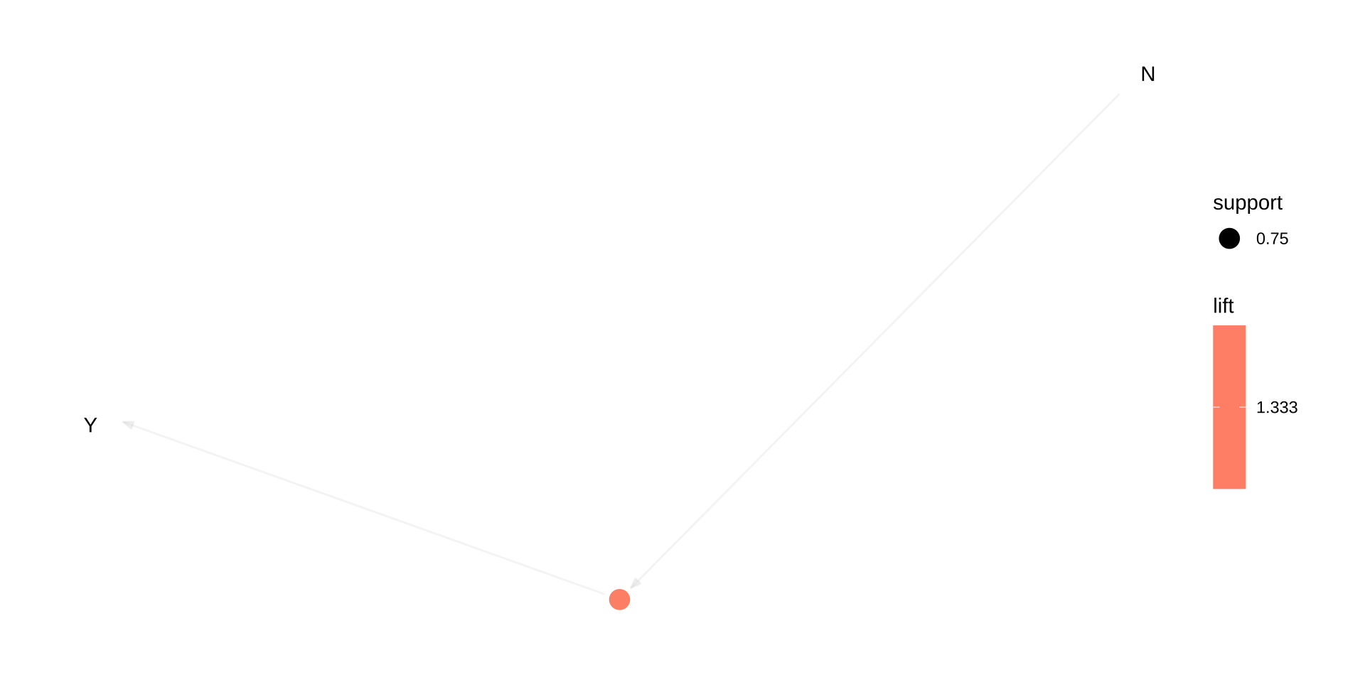    

plot(rules_N_lhs,method = "graph")

预期结果：

以 N 为前项的关联规则

规则	支持度	置信度	提升度	业务解读
{N} ⇒ {Y}	0.75	1.00	1.33	购买 N 的顾客中，100% 也购买了 Y
可考虑 N、Y 捆绑促销

提示

业务意义：在所有购买了 N 的顾客中，100% 都同时购买了 Y。这条规则支持度高（75%）、 置信度满分（100%），是制定捆绑促销策略的有力依据。

练习 8：以 N 为后项集的规则

目标：找出所有后项（rhs）中包含 N 的规则——"什么会引发对 N 的需求？"

# 筛选 rhs（后项）包含 N 的规则
rules_N_rhs <- apriori(trans,
                         parameter = list(support = 0.5,
                                          confidence = 0.8,
                                          target = "rules"),
                         appearance = list(rhs = c("N"),
                                           default = "lhs"))

Apriori

Parameter specification:
 confidence minval smax arem  aval originalSupport maxtime support minlen
        0.8    0.1    1 none FALSE            TRUE       5     0.5      1
 maxlen target  ext
     10  rules TRUE

Algorithmic control:
 filter tree heap memopt load sort verbose
    0.1 TRUE TRUE  FALSE TRUE    2    TRUE

Absolute minimum support count: 2 

set item appearances ...[1 item(s)] done [0.00s].
set transactions ...[5 item(s), 4 transaction(s)] done [0.00s].
sorting and recoding items ... [4 item(s)] done [0.00s].
creating transaction tree ... done [0.00s].
checking subsets of size 1 2 3 done [0.00s].
writing ... [2 rule(s)] done [0.00s].
creating S4 object  ... done [0.00s].

inspect(sort(rules_N_rhs, by = "lift"))

    lhs       rhs support confidence coverage lift  count
[1] {Y}    => {N} 0.75    1          0.75     1.333 3    
[2] {Y, Z} => {N} 0.50    1          0.50     1.333 2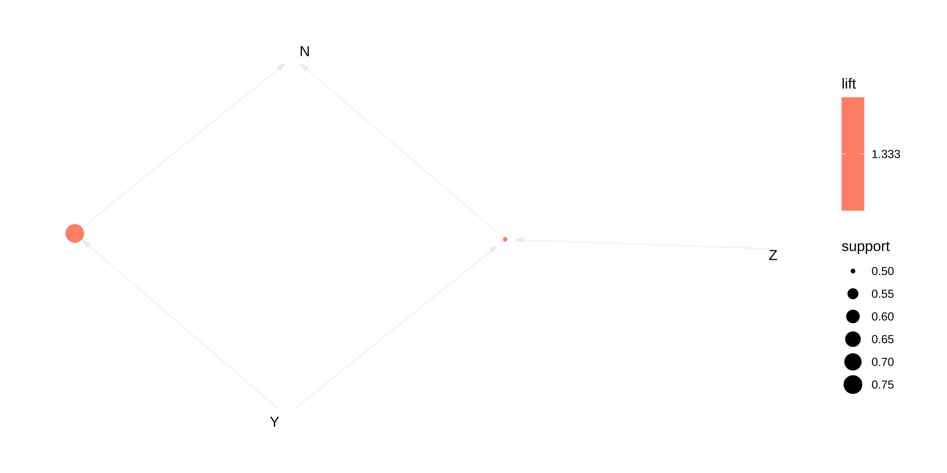    

plot(rules_N_rhs,method = "graph")

预期结果：

以 N 为后项的关联规则（按提升度排序）

规则	支持度	置信度	提升度	业务解读
{Y,Z} ⇒ {N}	0.50	1.00	1.33	购买 Y 和 Z 的顾客 100% 也买 N
{Y} ⇒ {N}	0.75	1.00	1.33	购买 Y 的顾客 100% 也买 N

提示

交叉销售建议：Y 是驱动 N 销售的关键前导商品。可以在 Y 的货架旁放置 N 的推荐标签， 或在顾客将 Y 加入购物车时，弹出 N 的关联推荐。

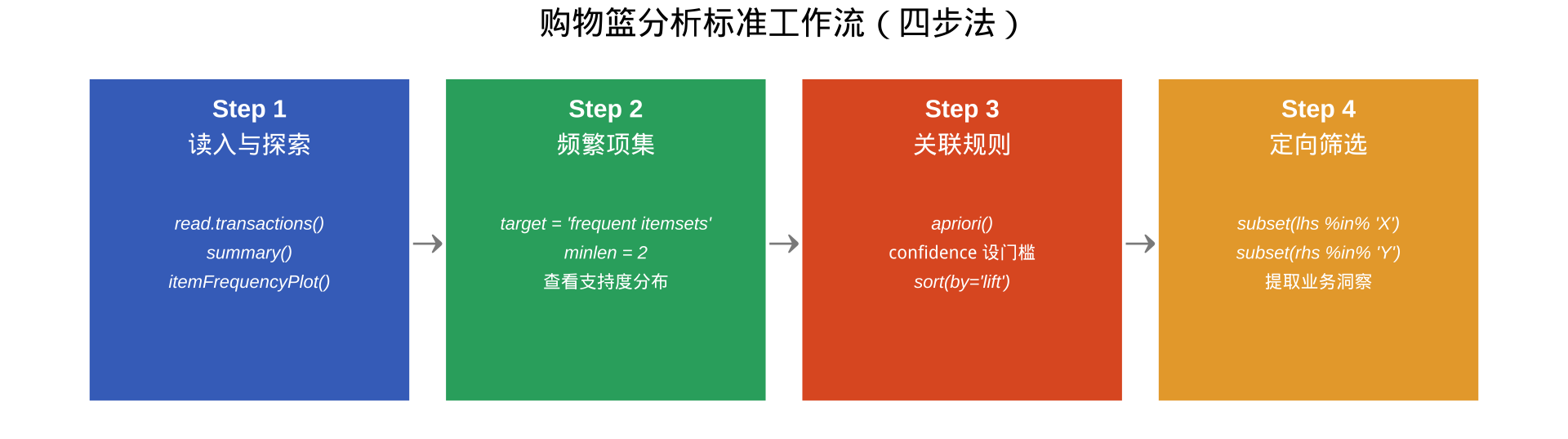
综合练习小结：四步分析框架

第 5 部分：课程总结

知识整合与下一步展望

本讲核心知识点回顾

关联规则完整方法论总结

• 三大度量（第 21 讲）：

  • 支持度（普遍性）→ 置信度（可靠性）→ 提升度（真实价值，最核心）
  • 提升度 < 1 的规则无论置信度多高都应丢弃

• Apriori 算法（第 21 讲）：反单调性剪枝，\(L_k \to C_{k+1} \to L_{k+1}\)，逐层迭代

• 参数调优（本讲）：support、confidence、minlen 三参数联合调节，先宽后严

• 精准筛选（本讲）：subset() 定向提取，sort(by="lift") 找最优规则

• 可视化（本讲）：散点图看全局 → 网络图看结构 → 业务决策

• 注意事项：关联 ≠ 因果；提升度优先于置信度；稀疏数据需降低 min_sup

关联规则的局限性与进阶方向

课后作业

加载 Groceries数据集，

library(arules)
library(arulesViz)
data("Groceries")
inspect(Groceries[1:20])

     items                      
[1]  {citrus fruit,             
      semi-finished bread,      
      margarine,                
      ready soups}              
[2]  {tropical fruit,           
      yogurt,                   
      coffee}                   
[3]  {whole milk}               
[4]  {pip fruit,                
      yogurt,                   
      cream cheese ,            
      meat spreads}             
[5]  {other vegetables,         
      whole milk,               
      condensed milk,           
      long life bakery product} 
[6]  {whole milk,               
      butter,                   
      yogurt,                   
      rice,                     
      abrasive cleaner}         
[7]  {rolls/buns}               
[8]  {other vegetables,         
      UHT-milk,                 
      rolls/buns,               
      bottled beer,             
      liquor (appetizer)}       
[9]  {pot plants}               
[10] {whole milk,               
      cereals}                  
[11] {tropical fruit,           
      other vegetables,         
      white bread,              
      bottled water,            
      chocolate}                
[12] {citrus fruit,             
      tropical fruit,           
      whole milk,               
      butter,                   
      curd,                     
      yogurt,                   
      flour,                    
      bottled water,            
      dishes}                   
[13] {beef}                     
[14] {frankfurter,              
      rolls/buns,               
      soda}                     
[15] {chicken,                  
      tropical fruit}           
[16] {butter,                   
      sugar,                    
      fruit/vegetable juice,    
      newspapers}               
[17] {fruit/vegetable juice}    
[18] {packaged fruit/vegetables}
[19] {chocolate}                
[20] {specialty bar}            

summary(Groceries)

transactions as itemMatrix in sparse format with
 9835 rows (elements/itemsets/transactions) and
 169 columns (items) and a density of 0.02609 

most frequent items:
      whole milk other vegetables       rolls/buns             soda 
            2513             1903             1809             1715 
          yogurt          (Other) 
            1372            34055 

element (itemset/transaction) length distribution:
sizes
   1    2    3    4    5    6    7    8    9   10   11   12   13   14   15   16 
2159 1643 1299 1005  855  645  545  438  350  246  182  117   78   77   55   46 
  17   18   19   20   21   22   23   24   26   27   28   29   32 
  29   14   14    9   11    4    6    1    1    1    1    3    1 

   Min. 1st Qu.  Median    Mean 3rd Qu.    Max. 
   1.00    2.00    3.00    4.41    6.00   32.00 

includes extended item information - examples:
       labels  level2           level1
1 frankfurter sausage meat and sausage
2     sausage sausage meat and sausage
3  liver loaf sausage meat and sausage

作业 1：参数敏感性分析

以0.01为支持度阈值，0.3为置信度阈值，挖掘以yogurt为后项集的关联规则

rules_yogurt_rhs <- apriori(
  data = Groceries, 
  parameter = list(
    support = 0.01,
    confidence= 0.3
  ),
  appearance = list(rhs = "yogurt"),
  control=list(verbose=F)
)

summary (rules_yogurt_rhs)

set of 9 rules

rule length distribution (lhs + rhs):sizes
2 3 
3 6 

   Min. 1st Qu.  Median    Mean 3rd Qu.    Max. 
   2.00    2.00    3.00    2.67    3.00    3.00 

summary of quality measures:
    support         confidence       coverage           lift          count    
 Min.   :0.0101   Min.   :0.313   Min.   :0.0261   Min.   :2.24   Min.   : 99  
 1st Qu.:0.0103   1st Qu.:0.324   1st Qu.:0.0305   1st Qu.:2.33   1st Qu.:101  
 Median :0.0109   Median :0.338   Median :0.0332   Median :2.42   Median :107  
 Mean   :0.0121   Mean   :0.341   Mean   :0.0358   Mean   :2.44   Mean   :119  
 3rd Qu.:0.0124   3rd Qu.:0.352   3rd Qu.:0.0397   3rd Qu.:2.52   3rd Qu.:122  
 Max.   :0.0173   Max.   :0.385   Max.   :0.0533   Max.   :2.76   Max.   :170  

mining info:
      data ntransactions support confidence
 Groceries          9835    0.01        0.3
                                                                                                                                          call
 apriori(data = Groceries, parameter = list(support = 0.01, confidence = 0.3), appearance = list(rhs = "yogurt"), control = list(verbose = F))

inspect(sort(rules_yogurt_rhs, by = "lift"))

    lhs                                       rhs      support confidence
[1] {whole milk, curd}                     => {yogurt} 0.01007 0.3852    
[2] {tropical fruit, whole milk}           => {yogurt} 0.01515 0.3582    
[3] {other vegetables, whipped/sour cream} => {yogurt} 0.01017 0.3521    
[4] {tropical fruit, other vegetables}     => {yogurt} 0.01230 0.3428    
[5] {whole milk, whipped/sour cream}       => {yogurt} 0.01088 0.3375    
[6] {citrus fruit, whole milk}             => {yogurt} 0.01027 0.3367    
[7] {curd}                                 => {yogurt} 0.01729 0.3244    
[8] {berries}                              => {yogurt} 0.01057 0.3180    
[9] {cream cheese }                        => {yogurt} 0.01240 0.3128    
    coverage lift  count
[1] 0.02613  2.761  99  
[2] 0.04230  2.568 149  
[3] 0.02888  2.524 100  
[4] 0.03589  2.457 121  
[5] 0.03223  2.420 107  
[6] 0.03050  2.413 101  
[7] 0.05328  2.326 170  
[8] 0.03325  2.280 104  
[9] 0.03965  2.242 122  

作业 2：针对后项为yogurt的关联规则结果，请截图得到的所有规则，并针对提升度最高的一条结果进行规则解读。

当顾客购买了（ ）且购买了（）时，他/她也会购买yogurt的概率是（）。

作业 3：以0.02为支持度阈值，0.4为置信度阈值，挖掘以whole milk为后项集的关联规则规则

rules_milk_rhs <- apriori(
  data = Groceries, 
  parameter = list(
    support = 0.02,
    confidence= 0.4
  ),
  appearance = list(rhs = "whole milk"),
  control=list(verbose=F)
)

summary(rules_milk_rhs)

set of 12 rules

rule length distribution (lhs + rhs):sizes
 2  3 
10  2 

   Min. 1st Qu.  Median    Mean 3rd Qu.    Max. 
   2.00    2.00    2.00    2.17    2.00    3.00 

summary of quality measures:
    support         confidence       coverage           lift          count    
 Min.   :0.0204   Min.   :0.402   Min.   :0.0434   Min.   :1.57   Min.   :201  
 1st Qu.:0.0230   1st Qu.:0.411   1st Qu.:0.0514   1st Qu.:1.61   1st Qu.:226  
 Median :0.0268   Median :0.449   Median :0.0570   Median :1.76   Median :264  
 Mean   :0.0312   Mean   :0.451   Mean   :0.0706   Mean   :1.76   Mean   :307  
 3rd Qu.:0.0347   3rd Qu.:0.490   3rd Qu.:0.0800   3rd Qu.:1.92   3rd Qu.:342  
 Max.   :0.0560   Max.   :0.513   Max.   :0.1395   Max.   :2.01   Max.   :551  

mining info:
      data ntransactions support confidence
 Groceries          9835    0.02        0.4
                                                                                                                                              call
 apriori(data = Groceries, parameter = list(support = 0.02, confidence = 0.4), appearance = list(rhs = "whole milk"), control = list(verbose = F))

inspect(sort(rules_milk_rhs, by = "lift"))

     lhs                                    rhs          support confidence
[1]  {other vegetables, yogurt}          => {whole milk} 0.02227 0.5129    
[2]  {butter}                            => {whole milk} 0.02755 0.4972    
[3]  {curd}                              => {whole milk} 0.02613 0.4905    
[4]  {root vegetables, other vegetables} => {whole milk} 0.02318 0.4893    
[5]  {domestic eggs}                     => {whole milk} 0.02999 0.4728    
[6]  {whipped/sour cream}                => {whole milk} 0.03223 0.4496    
[7]  {root vegetables}                   => {whole milk} 0.04891 0.4487    
[8]  {frozen vegetables}                 => {whole milk} 0.02044 0.4249    
[9]  {margarine}                         => {whole milk} 0.02420 0.4132    
[10] {beef}                              => {whole milk} 0.02125 0.4050    
[11] {tropical fruit}                    => {whole milk} 0.04230 0.4031    
[12] {yogurt}                            => {whole milk} 0.05602 0.4016    
     coverage lift  count
[1]  0.04342  2.007 219  
[2]  0.05541  1.946 271  
[3]  0.05328  1.919 257  
[4]  0.04738  1.915 228  
[5]  0.06345  1.850 295  
[6]  0.07168  1.760 317  
[7]  0.10900  1.756 481  
[8]  0.04809  1.663 201  
[9]  0.05857  1.617 238  
[10] 0.05247  1.585 209  
[11] 0.10493  1.578 416  
[12] 0.13950  1.572 551  

作业 4：针对后项为yogurt的关联规则结果，请截图得到的所有规则，并针对提升度最高的一条结果进行规则解读。

当顾客购买了（ ）且购买了（）时，他/她也会购买whole milk的概率是（）。

本讲小结

• 参数调优：support（频率）、confidence（可靠性）、minlen（规则长度）三参数联合调节；先宽松探索，再严格筛选；以 lift > 1 为基本准入门槛

• 精准筛选：subset(rules, lhs %in% "X") 找前项含 X 的规则，subset(rules, rhs %in% "Y") 找后项含 Y 的规则；sort(rules, by = "lift") 永远是第一步

• 可视化：散点图（整体分布）、网络图（关联结构）、分组矩阵图（系统梳理）；颜色深浅代表提升度，节点大小代表支持度

• 购物篮分析四步法：读入 → 频繁项集 → 关联规则 → 定向筛选 → 业务洞察

• 提升度是金标准：高置信度 + 提升度 < 1 = 无价值规则；高提升度才是真正值得关注的关联信号

谢谢！

第22讲：关联规则（二）——参数调优、可视化与购物篮分析实战

---

「找到规则容易，找到有价值的规则难——提升度就是那把过滤垃圾规则的筛子。」

---