Introduction to Survival Analysis in R
生存模型
1 Setup
2 Introduction
3 Kaplan-Meier estimator of the survival function
3.1 Kaplan-Meier estimation with survfit()
Call: survfit(formula = Surv(time, status) ~ 1, data = aml)

      n events median 0.95LCL 0.95UCL
[1,] 23 18 27 18 45# A tibble: 6 × 8
time n.risk n.event n.censor estimate std.error conf.high conf.low
<dbl> <dbl> <dbl> <dbl> <dbl> <dbl> <dbl> <dbl>
1 5 23 2 0 0.913 0.0643 1 0.805
2 8 21 2 0 0.826 0.0957 0.996 0.685
3 9 19 1 0 0.783 0.110 0.971 0.631
4 12 18 1 0 0.739 0.124 0.942 0.580
5 13 17 1 1 0.696 0.138 0.912 0.531
6 16 15 0 1 0.696 0.138 0.912 0.531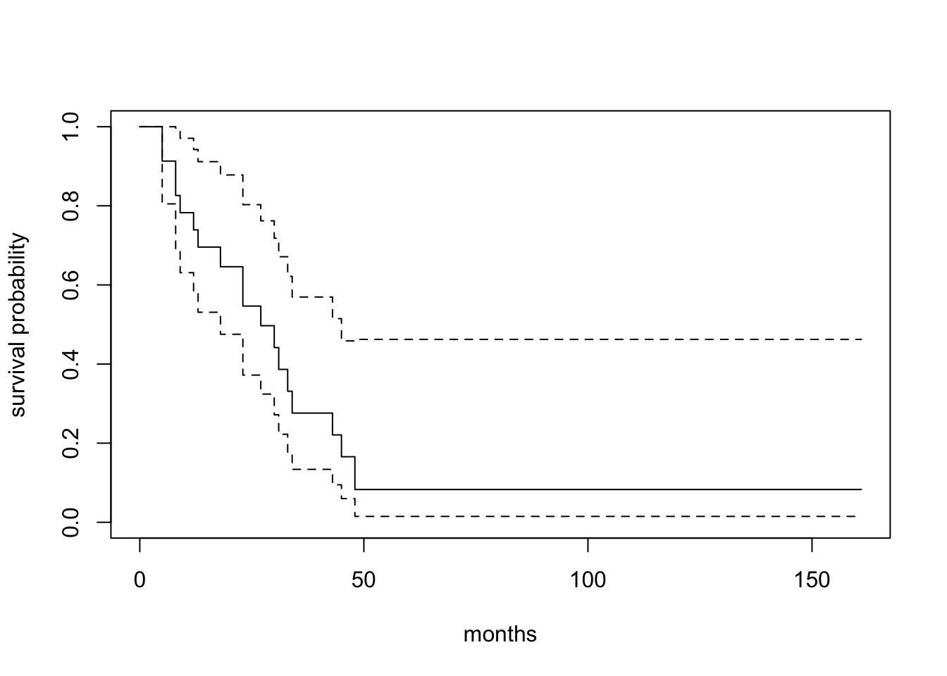
3.2 Stratified Kaplan-Meier estimates
Call: survfit(formula = Surv(time, status) ~ x, data = aml)

                 n events median 0.95LCL 0.95UCL
x=Maintained    11      7     31      18      NA
x=Nonmaintained 12 11 23 8 NA# A tibble: 6 × 9
time n.risk n.event n.censor estimate std.error conf.high conf.low strata
<dbl> <dbl> <dbl> <dbl> <dbl> <dbl> <dbl> <dbl> <chr>
1 9 11 1 0 0.909 0.0953 1 0.754 x=Maintai…
2 13 10 1 1 0.818 0.142 1 0.619 x=Maintai…
3 18 8 1 0 0.716 0.195 1 0.488 x=Maintai…
4 23 7 1 0 0.614 0.249 0.999 0.377 x=Maintai…
5 28 6 0 1 0.614 0.249 0.999 0.377 x=Maintai…
6 31 5 1 0 0.491 0.334 0.946 0.255 x=Maintai…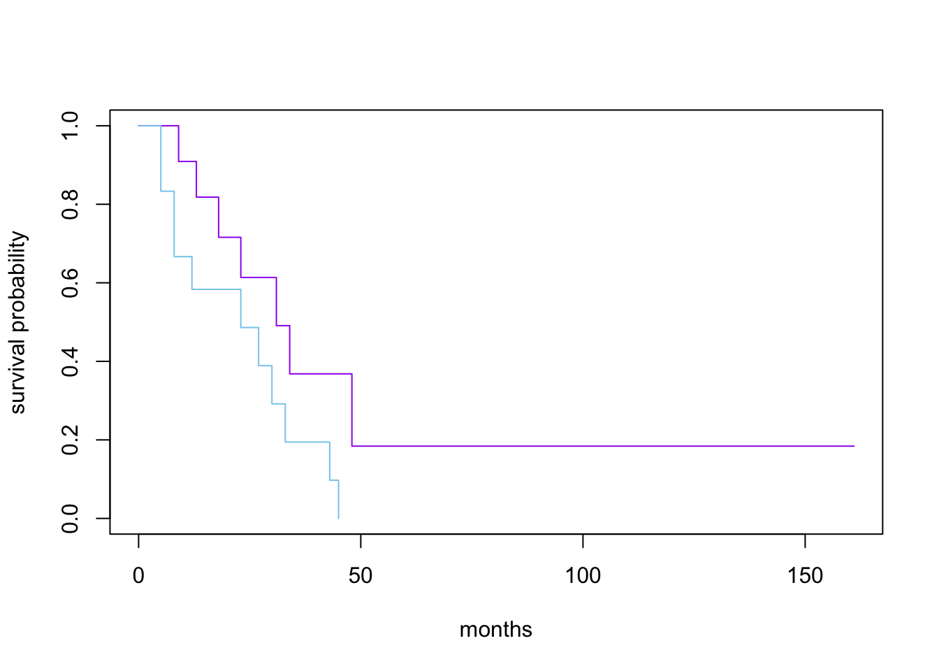
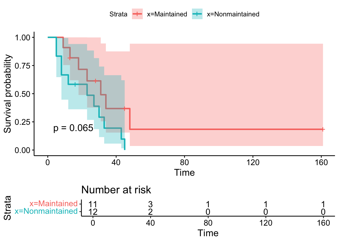
4 Comparing survival functions with survdiff()
We often want to test the hypothesis:
H0: survival curves across 2 or more groups are equivalent HA: survival curves across 2 or more groups are not equivalent
The log-rank statistic is one popular method to evaluate this hypothesis.
Under the null, the log-rank statistic is χ2 distributed with g−1 degrees of freedom.
The function survdiff() performs the log-rank test by default.
Call:
survdiff(formula = Surv(time, status) ~ x, data = aml)

                 N Observed Expected (O-E)^2/E (O-E)^2/V
x=Maintained    11        7    10.69      1.27       3.4
x=Nonmaintained 12       11     7.31      1.86       3.4

 Chisq= 3.4  on 1 degrees of freedom, p= 0.07
Code
Call:
survdiff(formula = Surv(time, status) ~ x, data = aml, rho = 1)

                 N Observed Expected (O-E)^2/E (O-E)^2/V
x=Maintained    11     3.85     6.14     0.859      2.78
x=Nonmaintained 12     7.18     4.88     1.081      2.78

Chisq= 2.8 on 1 degrees of freedom, p= 0.1 5 Exercise 1
The veteran data set describes survival times for veterans with lung cancer.
Variables:
time: survival time status: status, 0=censored, 1=dead trt: treatment, 1=standard, 2=test
- Create a graph and table of the Kaplan-Meier estimated survival function for the entire data set. What is the median survival time?
Call: survfit(formula = Surv(time, status) ~ 1, data = veteran)

       n events median 0.95LCL 0.95UCL
[1,] 137 128 80 52 105# A tibble: 6 × 8
time n.risk n.event n.censor estimate std.error conf.high conf.low
<dbl> <dbl> <dbl> <dbl> <dbl> <dbl> <dbl> <dbl>
1 1 137 2 0 0.985 0.0104 1 0.966
2 2 135 1 0 0.978 0.0128 1 0.954
3 3 134 1 0 0.971 0.0148 0.999 0.943
4 4 133 1 0 0.964 0.0166 0.995 0.933
5 7 132 3 0 0.942 0.0213 0.982 0.903
6 8 129 4 0 0.912 0.0265 0.961 0.866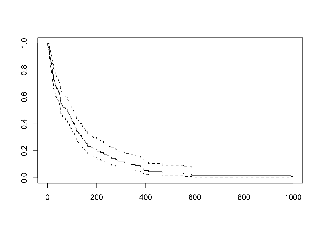
- Create a graph of KM estimated survival functions stratified by treatment, adding 95% confidence intervals and coloring the 2 functions. Does survival appear different for the 2 treatment groups?
Call: survfit(formula = Surv(time, status) ~ trt, data = veteran)

       n events median 0.95LCL 0.95UCL
trt=1 69     64  103.0      59     132
trt=2 68     64   52.5      44      95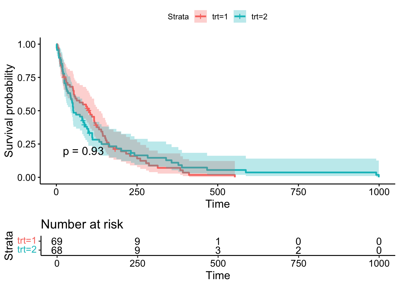
- Use the log-rank test to provide more evidence for your assessment of survival of the 2 groups.
6 The Cox proportional hazards model
6.1 Background
6.2 The Cox proportional hazards model
6.3 Proportional hazards
Fitting a Cox model
Call:
coxph(formula = Surv(time, status) ~ age + sex + wt.loss, data = lung)

  n= 214, number of events= 152
   (14 observations deleted due to missingness)

              coef  exp(coef)   se(coef)      z Pr(>|z|)
age      0.0200882  1.0202913  0.0096644  2.079   0.0377 *
sex     -0.5210319  0.5939074  0.1743541 -2.988   0.0028 **
wt.loss  0.0007596  1.0007599  0.0061934  0.123   0.9024
---
Signif. codes:  0 '***' 0.001 '**' 0.01 '*' 0.05 '.' 0.1 ' ' 1

        exp(coef) exp(-coef) lower .95 upper .95
age        1.0203     0.9801    1.0011    1.0398
sex        0.5939     1.6838    0.4220    0.8359
wt.loss    1.0008     0.9992    0.9887    1.0130

Concordance= 0.612  (se = 0.027 )
Likelihood ratio test= 14.67  on 3 df,   p=0.002
Wald test            = 13.98  on 3 df,   p=0.003
Score (logrank) test = 14.24  on 3 df,   p=0.003
6.4 Tidy coxph() results
# A tibble: 3 × 7
  term    estimate std.error statistic p.value conf.low conf.high
  <chr>      <dbl>     <dbl>     <dbl>   <dbl>    <dbl>     <dbl>
1 age        1.02    0.00966     2.08  0.0377     1.00      1.04
2 sex        0.594   0.174      -2.99  0.00280    0.422     0.836
3 wt.loss    1.00    0.00619     0.123 0.902      0.989     1.01
Code
lung.cox.tab |>
  ggplot(aes(
    x = estimate,
    y = term,
    xmin = conf.low,
    xmax = conf.high
  )) +
  geom_pointrange() +  # plots center point (x) and range (xmin, xmax)
  geom_vline(xintercept = 1, color = "purple") + # vertical line at HR=1
  labs(x = "hazard ratio", title = "Hazard ratios and 95% CIs") +
  theme_classic()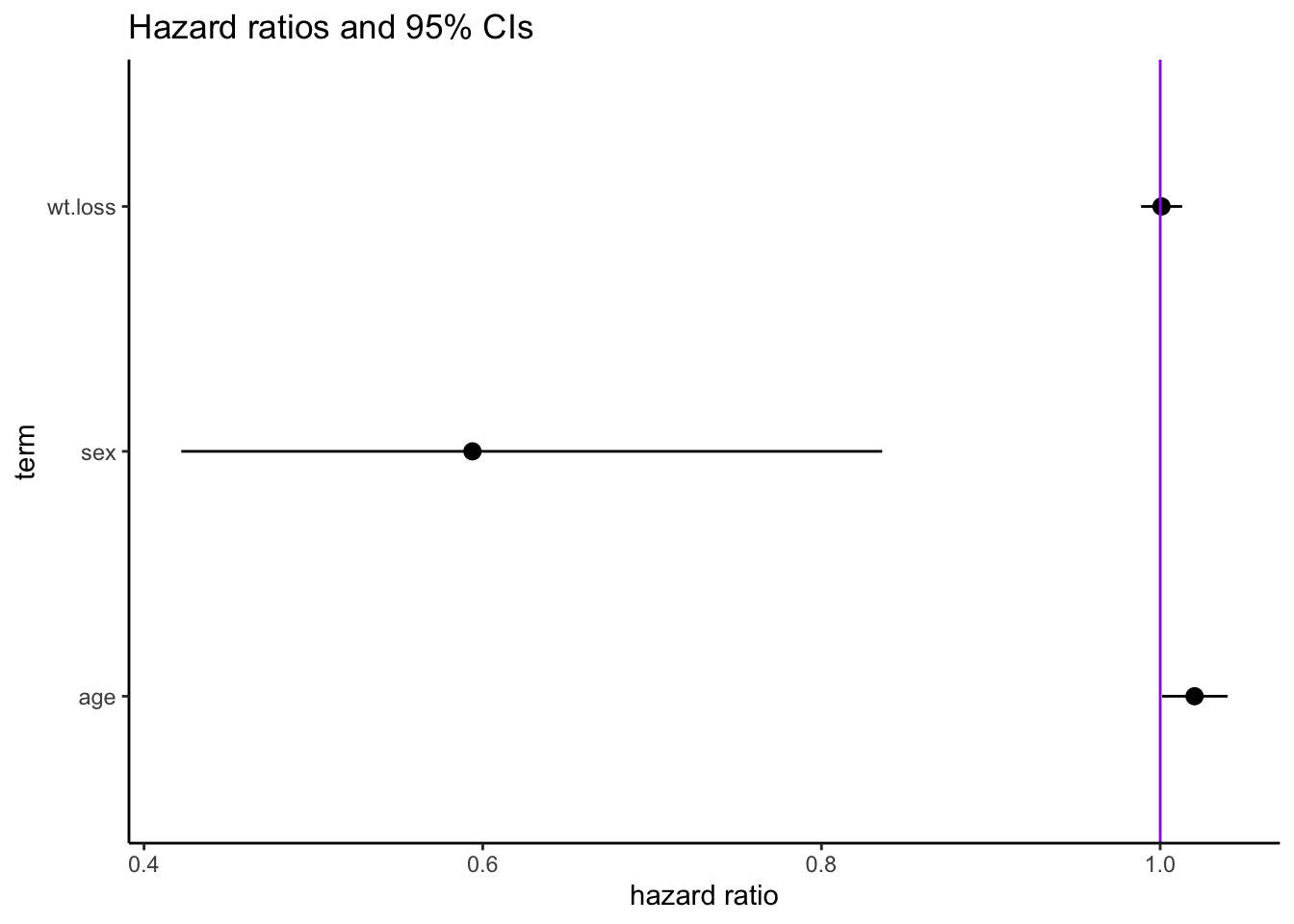
6.5 Predicting survival with Cox estimates
Code
# A tibble: 179 × 8
    time n.risk n.event n.censor estimate std.error conf.high conf.low
   <dbl>  <dbl>   <dbl>    <dbl>    <dbl>     <dbl>     <dbl>    <dbl>
 1     5    214       1        0    0.996   0.00443     1        0.987
 2    11    213       2        0    0.987   0.00772     1        0.972
 3    12    211       1        0    0.982   0.00894     1.00     0.965
 4    13    210       2        0    0.973   0.0110      0.995    0.953
 5    15    208       1        0    0.969   0.0120      0.992    0.946
 6    26    207       1        0    0.964   0.0128      0.989    0.940
 7    30    206       1        0    0.960   0.0137      0.986    0.935
 8    31    205       1        0    0.955   0.0145      0.983    0.929
 9    53    204       2        0    0.946   0.0160      0.976    0.917
10    54    202       1        0    0.942   0.0167      0.973    0.912
# ℹ 169 more rows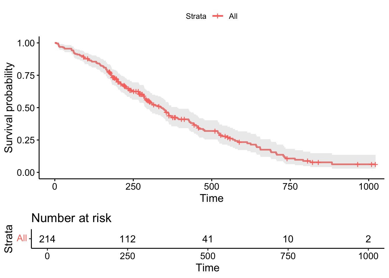
Code
       age sex  wt.loss
1 62.44737   1 9.831776
2 62.44737   2 9.831776
Code
# A tibble: 179 × 12
    time n.risk n.event n.censor estimate.1 estimate.2 std.error.1 std.error.2
   <dbl>  <dbl>   <dbl>    <dbl>      <dbl>      <dbl>       <dbl>       <dbl>
 1     5    214       1        0      0.995      0.997     0.00546     0.00327
 2    11    213       2        0      0.984      0.990     0.00953     0.00577
 3    12    211       1        0      0.978      0.987     0.0111      0.00674
 4    13    210       2        0      0.967      0.980     0.0137      0.00844
 5    15    208       1        0      0.962      0.977     0.0148      0.00921
 6    26    207       1        0      0.956      0.974     0.0159      0.00995
 7    30    206       1        0      0.951      0.971     0.0170      0.0107
 8    31    205       1        0      0.945      0.967     0.0180      0.0113
 9    53    204       2        0      0.934      0.960     0.0199      0.0127
10    54    202       1        0      0.929      0.957     0.0208      0.0133
# ℹ 169 more rows
# ℹ 4 more variables: conf.high.1 <dbl>, conf.high.2 <dbl>, conf.low.1 <dbl>,
#   conf.low.2 <dbl>
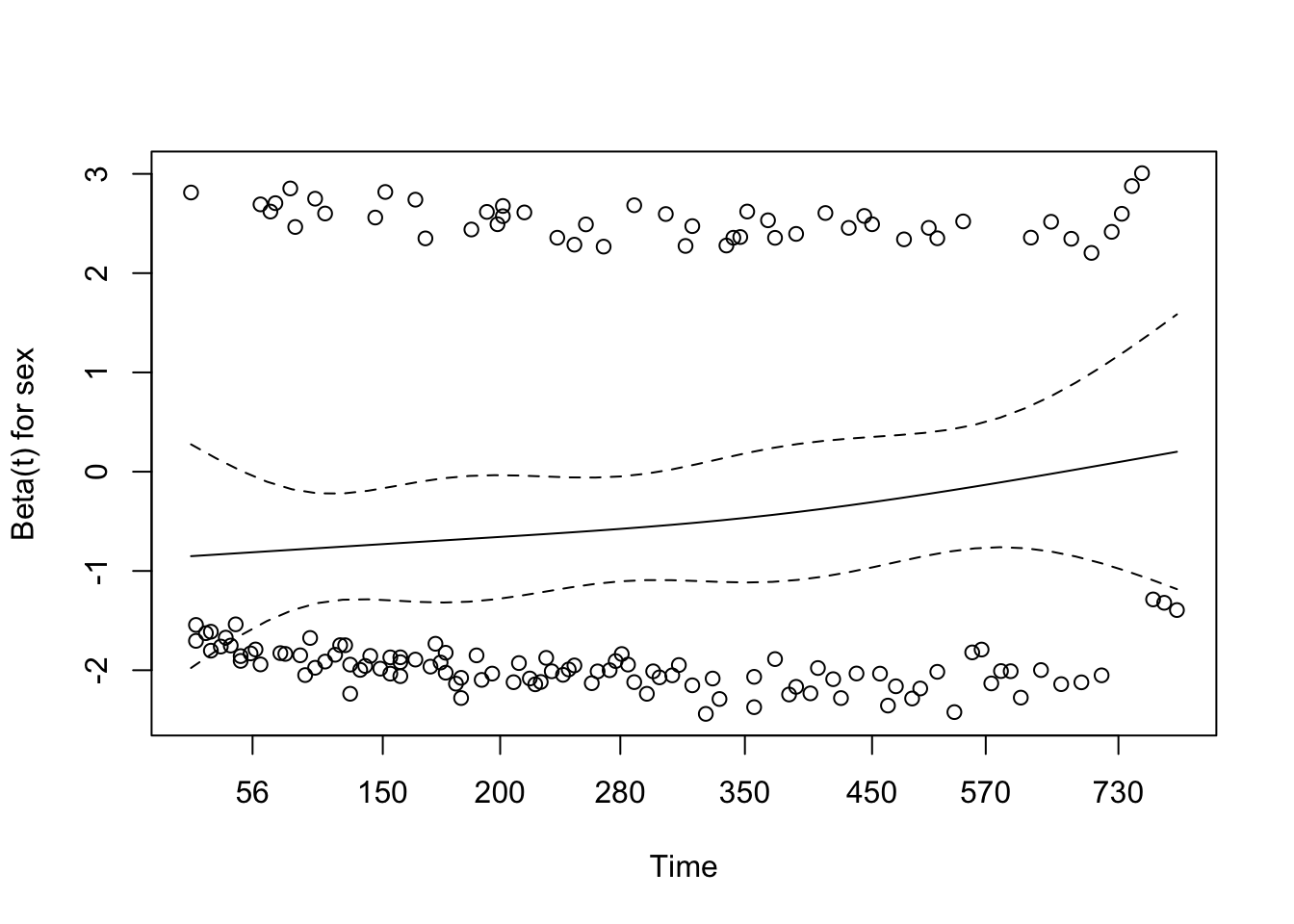
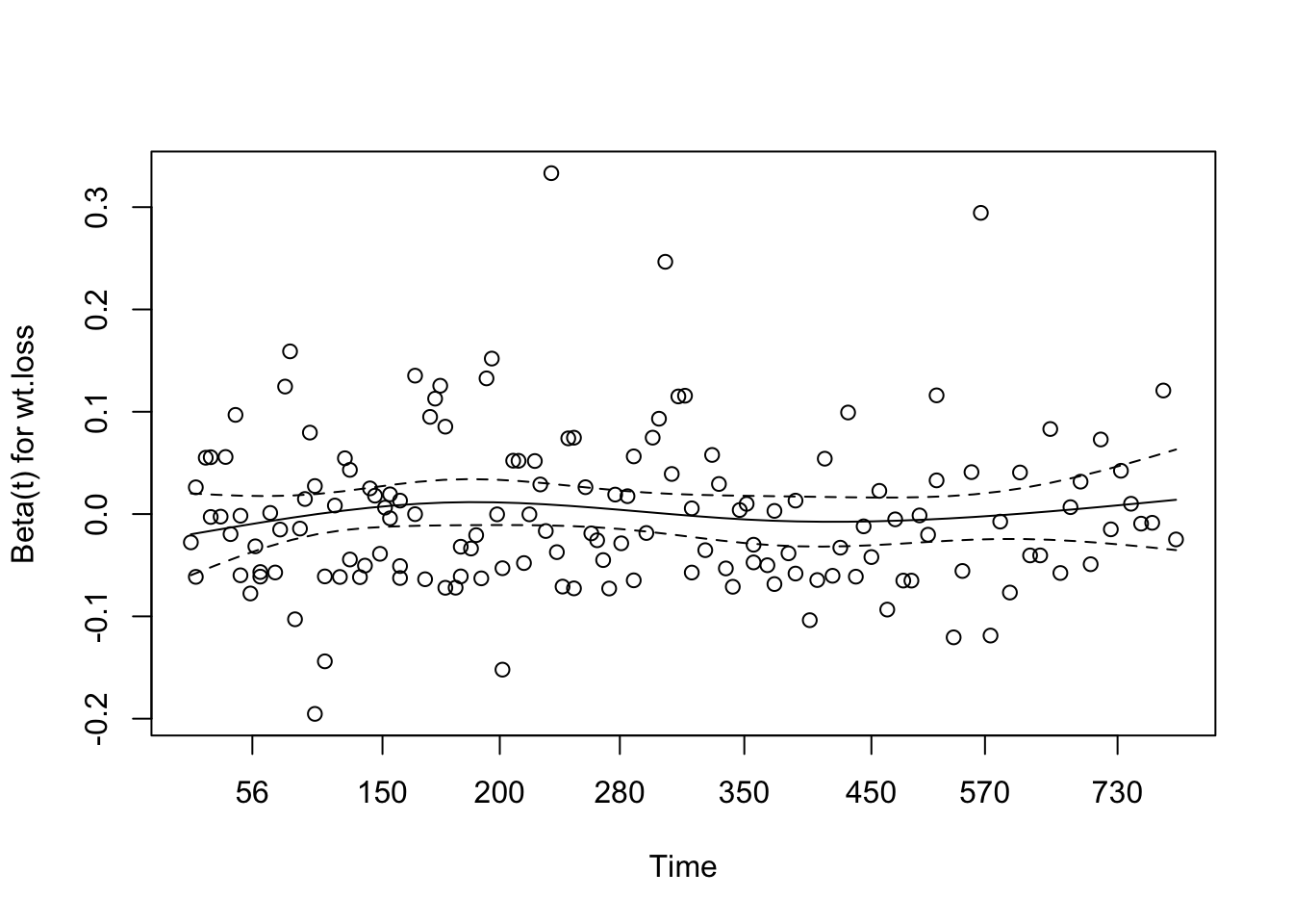
7 Assessing the proportional hazards assumption
A chi-square test based on Schoenfeld residuals is available with cox.zph() to test the hypothesis:
H0: covariate effect is constant (proportional) over time Ha: covariate effect changes over time
         chisq df    p
age     0.5077  1 0.48
sex     2.5489  1 0.11
wt.loss 0.0144  1 0.90
GLOBAL  3.0051  3 0.39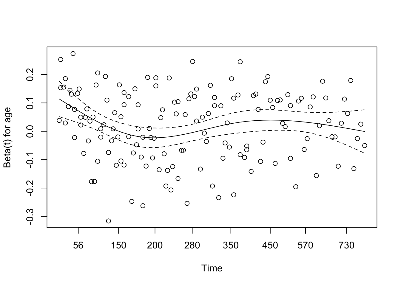
8 Dealing with proportional hazards violations
Call:
coxph(formula = Surv(time, status) ~ age + sex + wt.loss, data = lung)

  n= 214, number of events= 152
   (14 observations deleted due to missingness)

              coef  exp(coef)   se(coef)      z Pr(>|z|)
age      0.0200882  1.0202913  0.0096644  2.079   0.0377 *
sex     -0.5210319  0.5939074  0.1743541 -2.988   0.0028 **
wt.loss  0.0007596  1.0007599  0.0061934  0.123   0.9024
---
Signif. codes:  0 '***' 0.001 '**' 0.01 '*' 0.05 '.' 0.1 ' ' 1

        exp(coef) exp(-coef) lower .95 upper .95
age        1.0203     0.9801    1.0011    1.0398
sex        0.5939     1.6838    0.4220    0.8359
wt.loss    1.0008     0.9992    0.9887    1.0130

Concordance= 0.612  (se = 0.027 )
Likelihood ratio test= 14.67  on 3 df,   p=0.002
Wald test            = 13.98  on 3 df,   p=0.003
Score (logrank) test = 14.24  on 3 df,   p=0.003
9 Stratified Cox model
Code
Call:
coxph(formula = Surv(time, status) ~ age + wt.loss + strata(sex),
    data = lung)

  n= 214, number of events= 152
   (14 observations deleted due to missingness)

             coef exp(coef)  se(coef)     z Pr(>|z|)
age     0.0192190 1.0194049 0.0096226 1.997   0.0458 *
wt.loss 0.0001412 1.0001412 0.0062509 0.023   0.9820
---
Signif. codes:  0 '***' 0.001 '**' 0.01 '*' 0.05 '.' 0.1 ' ' 1

        exp(coef) exp(-coef) lower .95 upper .95
age         1.019     0.9810     1.000     1.039
wt.loss     1.000     0.9999     0.988     1.012

Concordance= 0.561  (se = 0.027 )
Likelihood ratio test= 4.09  on 2 df,   p=0.1
Wald test            = 3.99  on 2 df,   p=0.1
Score (logrank) test = 4  on 2 df,   p=0.1
10 Modeling time-varying coefficients
Code
Call:
coxph(formula = Surv(time, status) ~ age + wt.loss + sex + tt(sex),
    data = lung, tt = function(x, t, ...) x * t)

  n= 214, number of events= 152
   (14 observations deleted due to missingness)

              coef  exp(coef)   se(coef)      z Pr(>|z|)
age      0.0194343  1.0196244  0.0096522  2.013   0.0441 *
wt.loss  0.0001260  1.0001261  0.0062502  0.020   0.9839
sex     -0.9417444  0.3899470  0.3224791 -2.920   0.0035 **
tt(sex)  0.0013778  1.0013787  0.0008581  1.606   0.1084
---
Signif. codes:  0 '***' 0.001 '**' 0.01 '*' 0.05 '.' 0.1 ' ' 1

        exp(coef) exp(-coef) lower .95 upper .95
age        1.0196     0.9808    1.0005    1.0391
wt.loss    1.0001     0.9999    0.9879    1.0125
sex        0.3899     2.5645    0.2073    0.7337
tt(sex)    1.0014     0.9986    0.9997    1.0031

Concordance= 0.613  (se = 0.027 )
Likelihood ratio test= 17.23  on 4 df,   p=0.002
Wald test            = 15.86  on 4 df,   p=0.003
Score (logrank) test = 16.44  on 4 df,   p=0.002
11 Time-varying covariates
Code
Call:
coxph(formula = Surv(start, stop, event) ~ transplant + age +
    surgery, data = jasa1)

  n= 170, number of events= 75

               coef exp(coef) se(coef)      z Pr(>|z|)
transplant  0.01405   1.01415  0.30822  0.046   0.9636
age         0.03055   1.03103  0.01389  2.199   0.0279 *
surgery    -0.77326   0.46150  0.35966 -2.150   0.0316 *
---
Signif. codes:  0 '***' 0.001 '**' 0.01 '*' 0.05 '.' 0.1 ' ' 1

           exp(coef) exp(-coef) lower .95 upper .95
transplant    1.0142     0.9860    0.5543    1.8555
age           1.0310     0.9699    1.0033    1.0595
surgery       0.4615     2.1668    0.2280    0.9339

Concordance= 0.599  (se = 0.036 )
Likelihood ratio test= 10.72  on 3 df,   p=0.01
Wald test            = 9.68  on 3 df,   p=0.02
Score (logrank) test = 10 on 3 df, p=0.02 chisq df p
transplant 0.118 1 0.73
age 0.897 1 0.34
surgery 0.097 1 0.76
GLOBAL 1.363 3 0.71Code
# plot predicted survival by transplant group at mean age and surgery=0
plotdata <- data.frame(transplant=0:1, age=-2.48, surgery=0)
surv.by.transplant <- survfit(jasa1.cox, newdata=plotdata)
ggsurvplot(surv.by.transplant, data=plotdata) # remember to supply data to ggsurvplot() for predicted survival after coxph()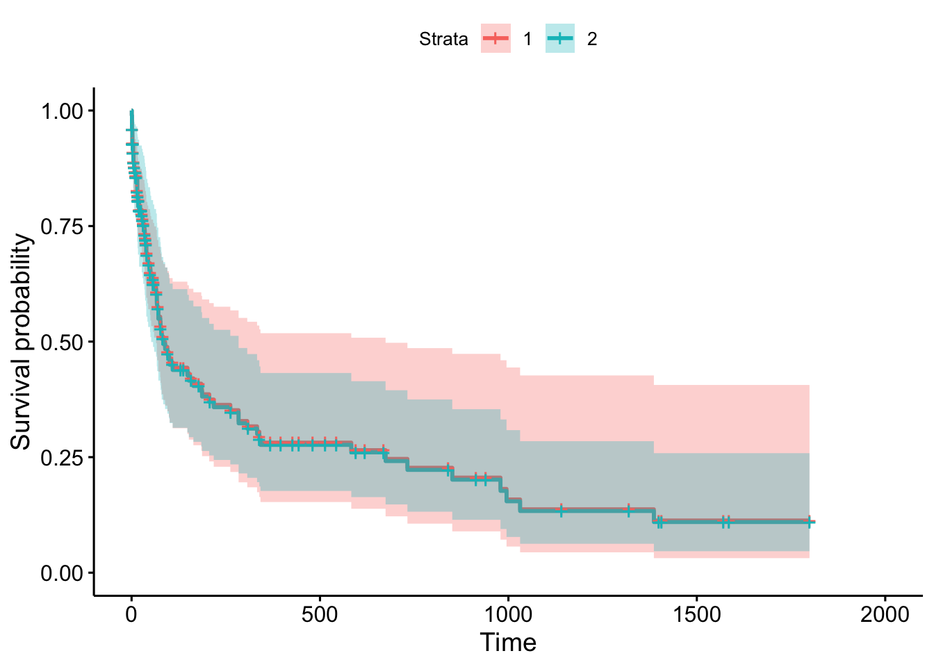
Code
Call:
coxph(formula = Surv(ST, State) ~ Group)

  n= 12, number of events= 12

         coef exp(coef) se(coef)     z Pr(>|z|)
GroupA 1.2515    3.4957   0.7227 1.732   0.0833 .
---
Signif. codes:  0 '***' 0.001 '**' 0.01 '*' 0.05 '.' 0.1 ' ' 1

       exp(coef) exp(-coef) lower .95 upper .95
GroupA     3.496     0.2861     0.848     14.41

Concordance= 0.652  (se = 0.072 )
Likelihood ratio test= 3.24  on 1 df,   p=0.07
Wald test            = 3  on 1 df,   p=0.08
Score (logrank) test = 3.36  on 1 df,   p=0.07